


1. Introduction
Vehicle routing problem was first proposed by G. Dantzig and J. Ramser in 1959 [1]. Once proposed, it attracted experts and scholars from mathematics, operations research, computer and other fields to research. At present, VRP problem is mostly solved by algorithms, which mainly includes exact algorithms [2] (such as: Branch and Bound Approach, Dynamic Planes Approach, Cutting Planes Approach, etc.) and heuristic algorithms. The heuristic algorithms also include traditional heuristic algorithms like Nearest-Neighbor Method, Clarke-Wright Saving Algorithm, etc. and meta-heuristic algorithms. The meta-heuristic algorithms are mainly referred to intelligence optimization algorithms like Tabu Search [3], Genetic Algorithm [4], etc. When the problems’ scale is constantly expanding, it is very difficult to find the optimal solution with the exact approaches. At present, the research on VRP by experts and scholars focuses on heuristic algorithms. The literature has proved that the standard vehicle routing problem is NP-hard combinatorial optimization problem, so the variant problems of different types of standard vehicle routing problems is also NP-hard combinatorial optimization problem. It is also challengingto construct more efficient algorithm for solving VRP.
In general, vehicle routing problems are described as follows: For a series of delivery points, a reasonable driving route is formed so that the vehicles pass through these points in an orderly manner. When meeting certain constraints (such as vehicle capacity, delivery or receiving time, distance limit, etc.), the driving route can reach some specific goals (such as the shortest driving route, the shortest time, the lowest cost, the highest profit, etc.). In practice, there are many different types of vehicle routing problems. Through the research and analysis of the literature in recent years, the vehicle routing problems can be divided into different types according to the different factors and constraints. According to whether there is a time window constraint, VRP can be divided into two types: the VRP with a time window (VRPTW) [5] and the VRP without a time window. Depending on the vehicle’s affiliation to the car park, it can be divided into two types: Open VRP (OVRP) [6] and closed vehicle routing problems. According to the type of vehicle, the problems can be divided into homogeneous vehicle routing problems and heterogeneous vehicle routing problems [7]. According to the number of car parks can be divided into single depot vehicle routing problems and multiple depot vehicle routing problems [8]. With the in-depth study of vehicle routing problem, many practical problems cannot be simply classified into a certain type, but more combinatorial problems that combine multiple constraints.
Bat Algorithm (BA) is a novel bionic algorithm proposed by Yang in 2010 [9]. This novel meta-heuristic optimization algorithm is inspired by the echolocation system of micro-bats. Bat algorithm has been widely concerned, because of its many advantages. For example, its algorithm model is simple, its parameter is less than the other algorithm, and it is easy to achieve. In recent years, many researchers have applied the bat algorithm to optimization problems and have made good progress. Bat algorithm shows better performance in many areas as follows: function optimization [10], image compression [11], combinatorial optimization [12], production scheduling [13], path planning [14] and so on. For all intelligence optimization algorithms, how to balance exploration and exploitation is a problem that we cannot ignore. Therefore, in this paper, we propose an improved bat algorithm with dynamic inertia weight and time factor. The dynamic inertia weight we used in this paper control every bats’ velocity dynamically, at the same time, time factor with weight adjustment for each generation of bats is added to avoid falling into the local optimum. Simulation results indicate that the improved bat algorithm shows excellent performance in solving multidimensional continuous space optimization problems. This paper applies the improved BA to solve Capacitated VRP (CVRP, abbreviation as VRP) [15], and demonstrates that the improved bat algorithm has achieved very good performance in solving discrete problems.
2. VRP Mathematical Model
Vehicle routing problems with capacity limitation are also referred to as standard vehicle routing problems, which means a maximum load capacity limit for each service vehicle. It is the most basic vehicle routing problem-- other variants of the vehicle routing problems are based on this. The general description of VRP is: Given a central warehouse and sub-warehouse, the location coordinates of each warehouse point and cargo demand ${{g}_{i}}(i=1, 2,\cdots , L)$ is known, the vehicle K loading capacity ${{q}_{k}}(k=1, 2,\cdots , K)$ is certain. Each car starts from the central warehouse to complete the distribution of the sub-warehouse and must return to the central warehouse after the task finished. If each sub-warehouse is accessed only once, the sum of the sub-warehouse visits required by each vehicle cannot exceed the vehicle loading capacity, and all sub-warehouse distributions need to be completed with minimum total cost.
According to the above description, the mathematical model of VRP can be established. The central warehouse number is 0, sub-warehouse number is $1, 2,\cdots , L,$ the demand for goods is${{g}_{i}}(i=1, 2,\cdots , L)$, vehicleKloading capacity is ${{q}_{k}}(k=1, 2,\cdots , K),$ the definition of variables are as follows:
${{y}_{ki}}=\left\{ \begin{matrix} 1,\text{ }sub-warehouse\text{ }i\text{ }task\text{ }by\text{ }the\text{ }vehicle\text{ }k \\ \text{0, }otherwise \\ \end{matrix} \right.$
${{x}_{ijk}}=\left\{ \begin{matrix} 1,\text{ }vehicle\text{ }k\text{ }from\text{ }i\text{ }to\text{ }j \\ \text{0, }otherwise \\ \end{matrix} \right.$
${{c}_{ij}}$ means transport costs that from point i to point j, actually its meaning can be distance, cost, time, and so on. In this paper, it represents the distance. The mathematical model of VRP is as follows: $X=({{x}_{ijk}})\in S$
$Min\text{ }Z=\sum\limits_{i}{\sum\limits_{j}{\sum\limits_{k}{{{c}_{ij}}{{x}_{ijk}}}}}$
In this model, the Equation (1) limits the carrying capacity of the vehicle. The Equation (2) ensures that each vehicle can be accessed by each customer only once. The Equation (3)-(5) form a loop. And Equation (6)-(7) is the defined variables. These Equations ensure that each sub-warehouse can get service, and the demand of each point can be completed by a car, while the total demand on each path does not exceed the load capacity of the vehicle. The objective function is fulfilled under such conditions - minimizing the sum of all vehicle travel paths.
As a NP-hard problem, VRP is difficult to solve. Since the issue was put forward, a considerable number of experts and scholars have conducted a great deal of research and laid the foundation for further research in the future.
3. BA and Improved BA
3.1. BA
The bat algorithm is an iterative-based optimization algorithm, similar to most meta-heuristic optimization algorithms. The bionic principle is that the bats are mapped to points in the search space, the search and optimization process is simulated as bats individual searching for prey and moving process. The objective function of the problem is measured as the pros and cons of the bat, the individual survival of the fittest process is simulated as the iterative process which is using better feasible solution to replace poor feasible solutionin the optimization process.
It is worth pointing out that the bat algorithm is not just a meta-heuristic algorithm. Compared with the existing meta-heuristic algorithm, it has two advantages: adaptive frequency adjustment and dynamic control of the detection in the global optimization and local optimization free switching. It simulates bat behavior using frequency-based tuning and pulse-rate-of-change, which gives the bat algorithm good convergence and is easier to implement than other algorithms. Bat algorithm uses dynamic search strategy. Like bats in prey on the automatic alignment, pulse emission rate and loudness changes automatically control the search behavior. In fact, when approaching to optimal, switching from local optimization to global optimization automatically can be achieved, therefore, the algorithm can be very effective in practice application problem.
In order to imitate this echolocation system of the micro-bats, Yang (2010) [3] have consider three appropriate and idealized rules as follows:
(1) All bats can use echolocation system to determine the distance, and can distinguish prey or obstacle in some way we cannot imagine;
(2) Bats fly randomly with velocity vi at position xi with a frequency f, wavelength $\lambda $ and loudness A0 to search for prey. They can automatically adjust the wavelength and frequency of their emitted pulses and adjust the rate $r\in [0,1]$ of pulse emission depending on the proximity of target;
(3) Although the loudness can vary in many ways, we assume that the loudness varies from a large A0 to a minimum constant value ${{A}_{\min }}$.
The optimization process of bats in BA can be described as follows:
Every bat is randomly distributed in the search space, their location is ${{x}_{i}}(i=1, 2,\cdots , N)$. Bats can emit ultrasonic pulses with frequency ${{f}_{i}}$, loudness A0 to search prey. Once confirming the target, they will fly to prey at velocity ${{v}_{i}}$, and then adjust the velocity, pulse rate and loudness based on the distance from target. According to the process, Yang designed the standard BA’s mathematical model, let t for iteration of the algorithm, i for each bat, ${{f}_{i}}$ for frequency that the bat iemitting, vi for velocity, xi for the location of bats. Therefore, the frequency, velocity and location updating Equation (8)-(10) is as follows:
In Equation (8), $\beta $ is a randomly generated number within the interval [0,1]. In general, the frequency f in a range $[{{f}_{\min }},{{f}_{\max }}]$ corresponds to a range of wavelengths $[{{\lambda }_{\min }},{{\lambda }_{\max }}]$. For example, a frequency range of [20kHz, 500kHz] corresponds to a range of wavelengths from 0.7mm to 1.7mm(Yang2010).
Actually, we can use any wavelength depending on different problems. The bats can adjust the range with the changing of frequency. In Equation (9), ${{x}_{*}}$ denotes the current global optimal solution gradually, they take local search strategy, using local solution updating Equation (11) as follows:
${{x}_{old}}$ denotes the solution of the current optimal solution, and $\varepsilon$ denotes a random number in the range [-1,1], while ${{A}^{t}}$ is the average loudness of all the bats at time t. Furthermore, with the iterations proceeding, the loudness ${{A}_{i}}$ and the rate ${{r}_{i}}$ of pulse emission must be updated based on these Equations (12) and (13).
Where $\alpha $ and $r$ are constants, for any $0<\alpha <1$ and $\gamma >0$, we can see that the loudness, ${{A}_{i}}$, decreases and the pulse rate, ${{r}_{i}}$, increases at the same time when the bats are near the prey step by step. In the simplicity case, the emission pulse rate, ${{r}_{i}}$, and loudness, ${{A}_{i}}$, are often randomly chosen at the first step, and the parameter $\alpha $ and $r$ set to 0.9 generally.
Above all, we can summarize BA’s two main strategies—exploration and exploitation. The former means global search strategy. When bats search for prey, its sound frequency is lower and the wavelength is longer and louder. The latter means local search strategy. When bats detect prey, its sound frequency is higher and the wavelength is shorter and quieter. This process will be repeated until the termination criteria met. The standard BA pseudo code is as follows.
Bat algorithm pseudo code
| Input: Initialize the bat population ${{x}_{i}}$, ${{f}_{i}}$, and ${{v}_{i}}$,$(i=1, 2,\cdots , n)$ |
|---|
| 1. While$(t<{{T}_{\max }})$; |
| 2. Update velocities and locations; |
| 3. If$(rand>{{r}_{i}})$; |
| Select a current best solution randomly among the best solutions and generate a local solution around the selected best solution; |
| 5. End if; |
| 6. Generate a new solution randomly; |
| 7. If ($rand<{{A}_{i}}$ and $f({{x}_{i}})<f({{x}_{*}})$); |
| 8. $f({{x}_{*}})=f({{x}_{i}})$; |
| 9. Increase ${{r}_{i}}$and reduce ${{A}_{i}}$; |
| 10. End if; |
| 11. Rank the bats and find the current best ${{x}_{*}}$; |
| 12. End while. |
3.2. Improved BA
Inspired by PSO’s dynamic inertia weight, this paper chooses a dynamic inertia weight based on Gaussion Normal Distribution [15-16]. Every generation, bats start searching from a random position with random velocity. With such a dynamic velocity, bats can be distributed throughout the search space immediately at a preliminary stage, which increases the opportunity to jump out of the local optimal solution bats fall into. According to this analysis, the modified velocity Equation (14) and dynamic inertia velocity Equation (15) is as follows:
Where ${{\omega }_{\max }}$ and ${{\omega }_{\min }}$ are the maximum $\omega$ value and minimum $\omega$ value, $rand()$ is a random number subjected to a uniform distribution in a range [0,1]. In this paper, $\sigma $ denotes the inertia deviation factor, in the range [0.1, 0.9], and is a random number subjected to a uniform distribution. In this Equation (14), using $\sigma \cdot normrnd()$ control deviation degree of inertia weight $\omega$. The $normrnd()$ is a random number subjected to Gaussion normal distribution in a range (0, 1). In short, such inertia weight not only makes the velocity of every generation of bats have randomness, but also have rationality. This enhances the diversity of bats in every generation and improves the BA’s convergence capability.
In physics, only two physical quantities with the same dimensions can be calculated directly. In the standard BA however, the position and velocity are directly added. Therefore, there is an implied time factor with a fixed value constant 1 in this Equation. This is the main reason why the bats vibrate near the optimal solution. So, we can change bat flight time randomly based on the iteration process to improve bat search ability.
According to the analysis above, this paper designs the time factor $t=0.1+\omega$, which is changed with the inertia weight change. In the improved bat algorithm, the bats can choose appropriate inertia weight and time factor self-adaptively based on the bat search feature during the iteration process to find the global optimal solution easily. The modified solution updating Equation is as follows-Equation (16):
4. Improved BA for VRP
4.1. The Basic Idea
First of all, the bat algorithm finds the optimal solution in an N-dimensional Hilbert space, and VRP is a typical discrete system optimization problem. The solution is obtained in the form of a sequence satisfying the constraints and the objective function. Using fast sort to map the points in N-dimensional Hilbert space into a solution vector, we can obtain the objective function value of this point by evaluating the cost of the sequence. In this process, each point in the search space corresponds to each bat in the bat algorithm, and the objective function value of each point is the fitness value of each bat.
4.2. Solution Code
In VRP, the central warehouse and sub-warehouses are discrete points, so the solution of real coding is adopted to convert the VRP into a quasi-continuous problem. In this way, the coding method is directly effective. In particular, the existing updating rules of the algorithm can be utilized directly in the running process and the algorithm can give full play to the advantages. The operation dimension of the algorithm is consistent with the problem solving dimension. Suppose there are L sub-warehouses and K cars, then the dimension of VRP solution is $d=L+K-1$. Each individual bat and velocity vector corresponds to one $(L+K-1)$ dimension vector. In fact, the resulting path has $(L+K+1)$ elements, but in this program, code does not need to consider the first and the last two 0s in advance. They only need to add the first and last two 0s when the total path is obtained. This not only has no effect on the calculation of the fitness value of each bat and the search of the optimal solution, but also can reduce the solution dimension and improve the search speed appropriately.
For example, the central warehouse code is 0, sub-warehouse code is $1, 2,\cdots , n$, and there are K vehicles involved in distribution. According to the mathematical model described above, if there are 10 sub-warehouses and 3 vehicles involved in distribution, you can get the form of the solution shown below (Figure 1).
Figure 1.
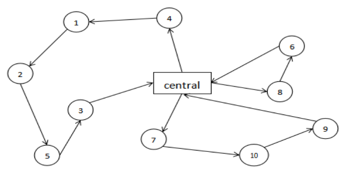
Figure 1.
Paths
Sub-path: Vehicle 1 Path: 0-4-1-2-5-3-0.
Vehicle 2 path: 0-7-10-9-0.
Vehicle 3 path: 0-8-6-0.
The total path: 0-4-1-2-5-3-0-7-10-9-0-8-6-0.
4.3. Steps
Step 1 Randomly initialize the bat population individual number N, frequency’s maximum value ${{f}_{\max }}$ minimum value ${{f}_{\min }}$, velocity ${{v}_{i}}$, location ${{x}_{i}}$, loudness $A_{i}^{t}$ and pulse rate ${{r}_{i}}$.
Step 2 Use fast sort to map the individual bat into a solution vector.
Step 3 Evaluate the feasibility of each solution vector, if feasible, switch to step 4, if not, switch to step 2.
Step 4 Based on fitness function $f(x)$,$x={{({{x}_{1}},{{x}_{2}},\cdots ,{{x}_{N}})}^{T}}$, find every bat fitness value and current optimal solution, record the bat current optimal location as ${{x}_{*}}$.
Step 5 Update velocity and location using (8),(14),(15).
Step 6 Generate a random number, if $rand>{{r}_{i}}$, generate ${{x}_{new}}$ around the selected best solution using (11).
Step 7 Generate a random number, if $rand>{{A}^{t}}$ and $f({{x}_{i}})<f({{x}_{*}})$,record ${{x}_{new}}$ as ${{x}_{best}}$, then update loudness $A_{i}^{t}$ and pulse rate ${{r}_{i}}$ using (12),(13).
Step 8 Evaluate fitness value, select best solution ${{x}_{*}}$ in this generation.
Step 9 Repeat the iteration process of step2 to step6, until finding global optimal solution or satisfying the maximum iteration number.
Step 10 Output global optimal solution.
5. Experiment
5.1. Example 1
For one central warehouse and eight sub-warehouses distribution system, the demand for each sub-warehouse is d = [12121422]. The delivery capacity for per car is 8 (in t). The known center warehouse and sub-warehouse distance is shown as below (Table 1). This requires reasonable arrangements for driving routes, which means the shortest distance. The required number of vehicles is calculated according to the Equation given in [17].
${{g}_{i}}$ is for each sub-warehouse cargo demand, q is for the load, $\alpha $ is a random number between (0, 1), and [] is for the rounding function. In Example 1, the number of vehicles is 2.
Table 1. Distance and demand
| 0 | 1 | 2 | 3 | 4 | 5 | 6 | 7 | 8 | |
|---|---|---|---|---|---|---|---|---|---|
| 0 | 0 | 4 | 6 | 7.5 | 9 | 20 | 10 | 16 | 8 |
| 1 | 4 | 0 | 6.5 | 4 | 10 | 5 | 7.5 | 11 | 10 |
| 2 | 6 | 6.5 | 0 | 7.5 | 10 | 10 | 7.5 | 7.5 | 7.5 |
| 3 | 7.5 | 4 | 7.5 | 0 | 10 | 5 | 9 | 9 | 15 |
| 4 | 9 | 10 | 10 | 10 | 0 | 10 | 7.5 | 7.5 | 10 |
| 5 | 20 | 5 | 10 | 5 | 10 | 0 | 7 | 9 | 7.5 |
| 6 | 10 | 7.5 | 7.5 | 9 | 7.5 | 7 | 0 | 7 | 10 |
| 7 | 16 | 11 | 7.5 | 9 | 7.5 | 9 | 7 | 0 | 10 |
| 8 | 8 | 10 | 7.5 | 15 | 10 | 7.5 | 10 | 10 | 0 |
| d | 1 | 2 | 1 | 2 | 1 | 4 | 2 | 2 | |
We used the improved bat algorithm proposed in this paper to solve the problems shown above. Each individual bat is mapped into a 9-dimensional (8+2-1) solution vector to represent the vehicle routing scheme. In this experiment, wehave run the improved bat algorithm 20 times, and the parameters’ setting is as followed:
Table 2. Solution for 20 times
| Algorithm | Times | |||||||||
|---|---|---|---|---|---|---|---|---|---|---|
| 1 | 2 | 3 | 4 | 5 | 6 | 7 | 8 | 9 | 10 | |
| Improved BA | 67.50 | 69.00 | 67.50 | 69.00 | 67.50 | 69.00 | 67.50 | 70.00 | 69.00 | 69.00 |
| 11 | 12 | 13 | 14 | 15 | 16 | 17 | 18 | 19 | 20 | |
| Improved BA | 67.50 | 70.00 | 67.50 | 69.00 | 69.50 | 70.00 | 69.00 | 67.50 | 67.50 | 69.00 |
Among them, the optimal solution is reached 8 times, the average value of solution is 68.575, and the optimal path is: 0→4→7→6→0→1→3→5→8→2→0. The total distance is 67.5.
Figure 2.
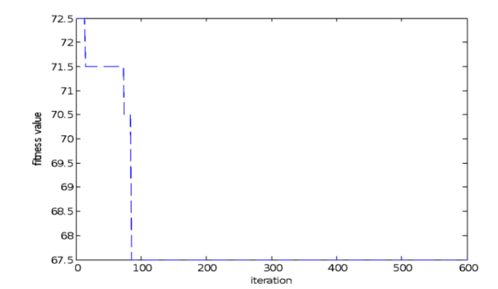
Figure 2.
Convergence curve
At the same time, it can be seen more intuitively through the convergence curve in
Table 3. Solution by standard GA and double-population GA for 10 times
| Algorithm | Times | |||||||||
|---|---|---|---|---|---|---|---|---|---|---|
| 1 | 2 | 3 | 4 | 5 | 6 | 7 | 8 | 9 | 10 | |
| standard GA | 74.00 | 75.00 | 71.50 | 72.00 | 73.50 | 75.00 | 73.00 | 72.50 | 75.50 | 73.50 |
| double-population GA | 70.00 | 69.50 | 67.50 | 71.00 | 69.00 | 70.50 | 72.00 | 67.50 | 71.50 | 69.00 |
| 11 | 12 | 13 | 14 | 15 | 16 | 17 | 18 | 19 | 20 | |
| standard GA | 72.00 | 69.00 | 73.00 | 75.50 | 72.00 | 73.00 | 75.00 | 73.50 | 71.50 | 75.00 |
| double-population GA | 67.50 | 69.00 | 71.00 | 70.00 | 67.50 | 70.50 | 69.00 | 69.50 | 71.00 | 69.00 |
It is known that the optimal solution of this problem is 67.5, the standard genetic algorithm reaches 0 times, the double population genetic algorithm reaches 4 times, and the improved bat algorithm reaches the known optimal solution 8 times. Thus, the improved bat algorithm can be used to solve the vehicle routing problem, and has good performance.
5.2. Example 2
We use the internationally VRP database benchmark test cases, the example 2(P-n19-k2) is downloaded from http://neo.lcc.uma.es/radi-aeb/WebVRP/index.html?/algorithms/clustRout.html/.
P-n19-k2 has 19 sub-warehouses, and coordinate and demand as shown in the following Table 4.
Table 4. P-n19-k2 coordinate and demand
| Coordinate | Demand | Coordinate | Demand | ||
|---|---|---|---|---|---|
| 0 | (30, 40) | 0 | 10 | (42, 57) | 8 |
| 1 | (37, 52) | 19 | 11 | (27, 68) | 7 |
| 2 | (49, 43) | 30 | 12 | (43, 67) | 14 |
| 3 | (52, 64) | 16 | 13 | (58, 27) | 19 |
| 4 | (31, 62) | 23 | 14 | (37, 69) | 11 |
| 5 | (52, 33) | 11 | 15 | (61, 33) | 26 |
| 6 | (42, 41) | 31 | 16 | (62, 63) | 17 |
| 7 | (52, 41) | 15 | 17 | (63, 69) | 6 |
| 8 | (57, 58) | 28 | 18 | (45, 35) | 15 |
| 9 | (62, 42) | 14 |
1is for the central warehouse, (1,
Table 5. Solution of P-n19-k2 for 10 times and the average value, standard deviation
| 1 | 2 | 3 | 4 | 5 | 6 | 7 | 8 | 9 | 10 | AV | Std | |
|---|---|---|---|---|---|---|---|---|---|---|---|---|
| P-n19-k2 | 288 | 265 | 266 | 258 | 282 | 265 | 272 | 275 | 274 | 284 | 272.9 | 2.83 |
The current best solution to this problem is known 212, The optimal path is as follows:
Vehicle 1 Path: 0-4-11-14-12-3-17-16-8-6-0.
Vehicle 2 path: 0-18-5-13-15-9-7-2-10-1-0.
It can be seen from the above results that the improved bat algorithm can be very close to the optimal solution. The solution efficiency and solution accuracy are higher than the standard bat algorithm.
6. Conclusion
The vehicle routing problem is an important part of the logistics distribution system, a reasonable way to determine the delivery path is very important to improve service quality. In this paper, a new real number coding scheme is designed, which transforms the discrete VRP into a quasi-continuous problem and is combined with the improved bat algorithm to solve the vehicle routing problem. The experiments show that the improved bat algorithm has its advantages, such as less parameters, easy implementation and so on, which can effectively solve VRP. However, the research in this paper is not perfect. It has been found in a large number of case experiments that the number of algorithm population andpopulation mutation rate also have a great influence on the solution. In the future, research can continue based on this research direction.
Acknowledgements
This work is supported by the Science & Technology Program of Henan Province, China (Grant No. 182102310886 and 162102110109). The authors would like to thank the anonymous reviewers and the editor for their helpful comments.
Reference
“The Truck Dispatching Problem, ”
“Exact Algorithms for the Vehicle Routing Problem based on Spanning Tree and Shortest Path Relaxations, ”
“Tabu Search, ”
“Genetic Algorithm in Search Optimization and Machine Learning, ”
“A Multiple Ant Colony System for Vehicle Routing Problems with Time Windows
”
“A Tabu Search Algorithm for the Open Vehicle Routing Problem, ”
“A Column Generation Approach to the Heterogeneous Fleet Vehicle Routing Problem, ”
“Heuristic Algorithms for Single and Multiple Depot Vehicle Routing Problems with Pickups and Deliveries, ”
“A New Metaheuristic Bat-Inspired Algorithm, ”
“Bat Algorithm for Multi-Objective Optimization, ”
“Fast Vector Quantization using a Bat algorithm for Image Compression, ”
“New Directional Bat Algorithm for Continuous Optimization Problems, ”
“Solving Multi-Stage Multi-Machine Multi-Product Scheduling Problem using Bat Algorithm, ”
“Three-Dimensional Path Planning for UCAV using an Improved Bat Algorithm, ”
“Separating Capacity Constraints in the CVRP using Tabu Search, ”
“Tracking and Optimizing Dynamic Systems with Particle Swarms
”DOI:10.1109/CEC.2001.934376 URL [Cited within: 1]
“A Modified Particle Swarm Optimizer, ”
“Genetic Algorithm for Vehicle Scheduling Problem with Non-Full Load, ”
