


Nomenclature
$S$ A multi-state system
$j$ Multi-state component
${{k}_{j}}$ Number of states of component $j$
${{G}_{j}}(t)$ Performance rate of component $j$at time $t$
${{u}_{j}}(z, t)$ UGF of component $j$ at time $t$
$u(z, t)$ UGF of $S$ at time $t$
$f$ Universal generating operator
${{f}_{ser}}$ Universal generating operator of series systems
${{f}_{par}}$ Universal generating operator of parallel systems
$K$ Number of states of $S$
${{L}^{n}}$ Performance rate space of $S$
${{S}_{1}}$ A flow transmission MSS
${{S}_{2}}$ A task processing MSS
${{T}_{j}}$ Task processing time of component j in ${{S}_{2}}$
$A(t, w)$ Availability
${{\delta }_{A}}$ Availability operator
$E(t)$ Mean output performance
${{\delta }_{E}}$ Mean output performance operator
$D(t, w)$ Mean output performance deficiency
${{\delta }_{D}}$ Mean output performance deficiency operator
${{\omega }_{j}}$ Weight of performance rate ${{G}_{j}}$
${{u}^{(1)}}(z)$ UGF of fixed-weight MSS
${{u}^{(2)}}(z)$ UGF of variable-weight MSS
$w$ System demand
$f(x)$ Probability density function of standardized normal distribution
$I({{g}_{i}}(t)\ge w)$ An indicator function
1. Introduction
In traditional reliability theory, we usually assume only two possible states for a system and its components: perfect functionality and complete failure. In other words, state 1 represents a system working well while 0 represents it failing. However, for most systems in real engineering, in addition to two states of perfect functionality and complete failure, there are also a series of deteriorating states [1-4]. For example, in a power generation system, when the generator generates a power of 100MW, the system is in a normal state, and when it generates a power of 0MW, the system is in a state of complete failure. However, due to some types of faults, the generated power may be 80MW at one time and 60MW at another time. These systems are called multi-state systems (MSSs). Actually, a binary system is the simplest multi-state system containing two distinctive states 1 and 0.
Since the concept of MSSs was proposed, many scholars have spread their research on the reliability of MSSs [5-7]. From qualitative assessment to quantitative analysis, from the same number of states to different numbers, and from an ordered set to a partially ordered set of the description of state space, four main methods of reliability evaluation for MSSs have been gradually formed: an extension of the Boolean model [8], stochastic process method [9], universal generating function (UGF) technology [10-12], and Monte-Carlo simulation [13]. Due to the advantages of convenient computation and easy analysis, UGF has been widely studied in reliability evaluation and optimization of MSSs. It has gradually become one of the most basic and commonly used methods for the reliability assessment of MSSs [2,14-15].
Based on the z-transform of discrete random variables, the state performance and corresponding possibility of multi-state components can be represented by au function. According to the connection structure between components and performance characteristics, we can design universal generating operators [16] and then obtain polynomial representation of the whole system. Finally, we can evaluate and optimize the reliability of MSSs combined with system demand. In the process of reliability evaluation of MSSs, universal generating operators have a significant influence on output performance and state probability of the whole system, which will affect the reliability of MSSs to a great extent.
In the process of reliability management, when the connection relationship between components is unknown and the system performance is uncertain [17], assigning a proper weight to the multi-state component performance and constructing a more general UGF will be important for evaluating and optimizing the reliability of MSSs. Therefore, on the basis of UGF, this paper introduces the Ordered Weighted Averaging (OWA) [18] operator into weight determination when calculating system output performance. By designing reliability evaluation indices of MSSs and constructing a weighted universal generating function, reliability parameters of MSSs [19-20] can be evaluated. The case starts from a steam turbine power generation system, proving the practicability of the method proposed in this paper through a comparison with the traditional universal generating function.
The organization of this paper is as follows. Section 2 describes the basic synthetic methods of system performance according to connection relationships between components and performance characteristics and then proposes three main reliability indices in the reliability evaluation of MSSs. Section 3 puts forward the definition of weighted universal generating function and establishes two methods of weight determination of system performance. In Section 4, for a steam turbine power generation system in a repairable naval equipment system where the connection structures between components are unknown, we use four styles of weighted universal generating function to evaluate the multi-state system’s reliability. Finally, we present conclusions of this paper in Section 5.
2. Universal Generating Function
2.1. System Performance Associated with Connection Structures Between Components
Suppose that an MSS $S$ has $n$ components and each component $j(j=1, 2,\cdots , n)$ has ${{k}_{j}}$ states. The performance rate of $j$ at time $t$ is ${{G}_{j}}(t)$ and ${{G}_{j}}(t)\in \{{{g}_{j1}}(t),{{g}_{j2}}(t),\cdots ,{{g}_{j{{k}_{j}}}}(t)\}$, the corresponding state probability is ${{P}_{j}}(t)$, and ${{P}_{j}}(t)\in \{{{p}_{j1}}(t),{{p}_{j2}}(t),\cdots ,{{p}_{j{{k}_{j}}}}(t)\}$. Then, the universal generating function of multi-state component $j$ is
The universal generating function of the multi-state system $S$ is
In Equation(2), $f$ is the system structure function and is also called the universal generating operator. In general, ${{f}_{ser}}$ is used to represent the series connection while ${{f}_{par}}$ is used to represent the parallel connection. From Equation (2), we can see that the number of states of multi-state system $S$ is
The performance rate space is ${{L}^{n}}=\{{{g}_{11}},{{g}_{12}},\cdots ,{{g}_{1{{k}_{1}}}}\}\times \{{{g}_{21}},{{g}_{22}},\cdots ,{{g}_{2{{k}_{2}}}}\}\times \cdots \times \{{{g}_{n1}},{{g}_{n2}},\cdots ,{{g}_{n{{k}_{n}}}}\}$. Suppose that the performance capability of $j(j=1, 2,\cdots , n)$ is ${{G}_{j}}$ and ${{G}_{j}}\in \{{{g}_{j1}},{{g}_{j2}},\cdots ,{{g}_{j{{k}_{j}}}}\},\text{(}j=1, 2,\cdots , n)$. There are two common types of MSS: flow transmission MSS and task processing MSS. For the series system ${{S}_{1}}$ constituted by multi-state components as shown in Figure 1(a), when ${{S}_{1}}$ is a flow transmission MSS and performance ${{G}_{j}}(j=1, 2,\cdots , n)$ represents the transmission capability, the total transition capability of ${{S}_{1}}$ depends on the bottleneck component.
Figure 1.
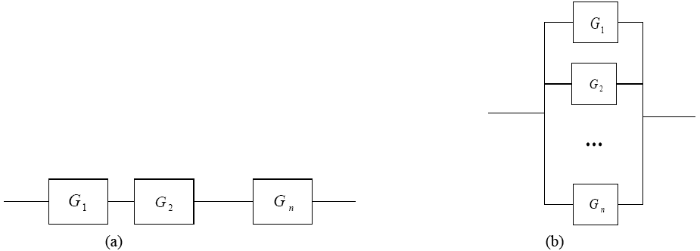
Figure 1.
(a) A multi-state series system; (b) A multi-state parallel system
When S1 is a task processing MSS and performance ${{G}_{j}},(j=1, 2,\cdots , n)$ represents the processing speed, the task processing time of component $j$ is ${{T}_{j}}=1/{{G}_{j}},\text{ }({{G}_{j}}\ne 0)$. The total performance rate is
For the parallel system ${{S}_{2}}$ constituted by multi-state components as shown in Figure 1(b), when ${{S}_{2}}$ is a flowtransmission MSS, the total performance rate of ${{S}_{2}}$ is
When ${{S}_{2}}$ is a task processing MSS, the total performance rate of ${{S}_{2}}$ is
Table 1. Relationship between system performance and component performances
| Type of MSS | System performance | |
|---|---|---|
| Series system | Flow transmission MSS | $G_{s}^{(1)}=\min \{{{G}_{1}},{{G}_{2}},\cdots ,{{G}_{n}}\}$ |
| Task processing MSS | $G_{s}^{(2)}=\frac{1}{\sum\limits_{j=1}^{n}{(1/{{G}_{j}})}}$ | |
| Parallel system | Flow transmission MSS | $G_{s}^{(3)}=\sum\limits_{j=1}^{n}{{{G}_{j}}}$ |
| Task processing MSS | $G_{s}^{(4)}=\max \{{{G}_{1}},{{G}_{2}},\cdots ,{{G}_{n}}\}$ |
From Table 1, we can see that the total performance rate ${{G}_{s}}$ can be regarded as a certain function relationship of ${{G}_{1}},{{G}_{2}},\cdots ,{{G}_{n}}$, that is,${{G}_{s}}=f({{G}_{1}},{{G}_{2}},\cdots ,{{G}_{n}})$.$f(\cdot )$isgenerally decided by the connection relationship between components and system performance characteristics. In the general series-parallel system shown in Figure 2, the relationship between${{G}_{s}}$ and ${{G}_{j}}(j=1, 2,\cdots , n)$ can be represented as
Figure 2.
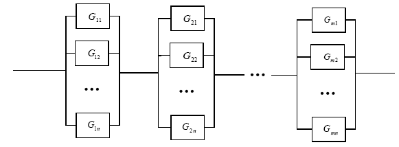
Figure 2.
A general series-parallel system
2.2. Reliability Evaluation Indices of MSSs
System reliability refers to the ability of a product to complete the prescribed function under specified conditions and time, and we often use time function $R(t)$ to measure the reliability of a system or a product. Suppose in a constant condition profile, the demand of an MSS is $w$ at time $t$. The system performance is${{G}_{s}}(t)\in \{{{g}_{1}}(t),{{g}_{2}}(t),\cdots ,{{g}_{K}}(t)\}$ and the corresponding possibility is${{P}_{s}}(t)\in \{{{p}_{1}}(t),{{p}_{2}}(t),\cdots ,{{p}_{K}}(t)\}$, in which $K$ is the total number of system performances and according to Equation (3),$K=\prod\limits_{j=1}^{n}{{{k}_{j}}}$. In general, the reliability measurement parameters include availability $A(t, w)$, mean output performance $E(t)$, and mean output performance deficiency $D(t, w)$.
Availability of an MSS $S$ is the possibility that the system performance satisfies the demand, namely,
In Equation (9), ${{\delta }_{A}}$ is called the availability operator, $I({{g}_{i}}(t)\ge w)$ is an indicator function, and
Then, Equation(9) can be transferred to
When $t\to +\infty $, we can obtain the stable availability of an MSS
The mean output performance $E(t)$ of an MSS $S$ is the average value of the system output performance, namely,
In Equation (13), ${{\delta }_{E}}$ is called the mean output performance operator. From Equation (13), we can see that the mean output performance $E(t)$of an MSS has nothing to do with the demand $w$.
When $t\to +\infty $, we can obtain the stable mean output performance of an MSS:
The mean output performance deficiency of an MSS is the average value when the system output performance does not satisfy demand, namely,
In Equation (15), ${{\delta }_{D}}$ is called the mean output performance deficiency operator. When $t\to +\infty $, we can obtain the stable mean output performance deficiency value of an MSS $S$:
3. Reliability Evaluation of Uncertain MSS
3.1. Weighted Universal Generating Function
From Equations (2) and (3), we can see that the total state numbers of an MSSis $K$, the system performance $f({{g}_{1{{j}_{1}}}}(t),{{g}_{2{{j}_{2}}}}(t),\cdots ,{{g}_{n{{j}_{n}}}}(t))$ is the function of each component performance, and we can use ${{g}_{k}}(k=1, 2,\cdots , K)$ to replace it. When the connection structure between components is unknown or the component performance appears to have uncertain characteristics, the total system performance ${{G}_{s}}\in \{{{g}_{1}},{{g}_{2}},\cdots ,{{g}_{K}}\}$ cannot be determined by Equations (4) to (8). Anyway, ${{G}_{s}}$ can be represented as the sum of the weighted performance of ${{G}_{1}},{{G}_{2}},\cdots ,{{G}_{n}}$, that is,
where $\sum\limits_{i=1}^{n}{{{\omega }_{i}}}=1$. Then, the weighted universal generating function (WUGF) can be defined as follows:
In an MSS, the performance of multi-state component $j(j=1, 2,\cdots , n)$ is ${{G}_{j}}$, and its universal generating function is shown in Equation (1). When the connection structure between components is unknown or the component performance appears to have uncertain characteristics, the weighted universal generating function (WUGF) of the whole system is
3.2. Determination of System Performance Weight
In the process of system performance determination, different weights are applied to component performances, which reflects the relative importance of each component in the MSS and will be more objective. Generally speaking, the weight determination methods include subjective experience, primary and secondary index queuing classification, expert survey, and so on. Different weight determination methods have greater impact on the final results of system reliability. The weight determination method based on the Ordered Weighted Averaging (OWA) operator is the most commonly used method in multi-attribute decision making, and it is widely used in every field such as production and life.
1)Fixed Weight Universal Generating Function
In order to reflect the principle of fairness, a greater weight should be applied to components with greater performance rate in an uncertain MSS [21]. That is, the weight ${{\omega }_{j}}$ of component $j(j=1, 2,\cdots , n)$ has relations with its performance rate ${{G}_{j}}\in \{{{g}_{j1}},{{g}_{j2}},\cdots ,{{g}_{j{{k}_{j}}}}\}$ and ${{\omega }_{j}}$ changes with ${{G}_{j}}$, as shown in Equation (19).
Here, the MSS composed of the fixed weight universal generating function is called fixed-weight MSS, namely,
Then, we can evaluate and optimize the reliability of a fixed weight MSS according to Equations (9) to (16) on the basis of system demand $w$.
2)Variable Weight Universal Generating Function
In literature [22], Xu proposed an OWA operator weight determination method based on normal distribution, and literature [23] improved this method starting from decision data. On the basis of considering performance data of a multi-state component, we will improve the OWA operator to determine the component performance weight by taking from the standardized normal distribution.
Suppose that an MSS contains $n$ components and the performance of component $j(j=1, 2,\cdots , n)$ is ${{G}_{j}}\in \{{{g}_{j1}},{{g}_{j2}},\cdots ,{{g}_{j{{k}_{j}}}}\}$. For performance vector $\overrightarrow{G}=({{G}_{1}},{{G}_{2}},\cdots ,{{G}_{n}})$, its expectation and standard deviation [24] are respectively
$\mu =\frac{1}{n}\sum\limits_{j=1}^{n}{{{G}_{j}}}$,$\sigma =\frac{1}{n}\sum\limits_{j=1}^{n}{{{({{G}_{j}}-\mu )}^{2}}}$
Then, after standardization of $\overrightarrow{G}=({{G}_{1}},{{G}_{2}},\cdots ,{{G}_{n}})$, we can obtain ${{\overrightarrow{G}}^{(s)}}=({{G}_{1}}^{(s)},{{G}_{2}}^{(s)},\cdots ,{{G}_{n}}^{(s)})$, in which
${{G}_{j}}^{(s)}=\frac{{{G}_{j}}-\mu }{\sigma }$
Suppose the probability density function of standardized normal distribution $N(0, 1)$ is $f(x)=\frac{1}{\sqrt{2\pi }}\exp (-\frac{{{x}^{2}}}{2})$ and the function value of standardized performance${{\overrightarrow{G}}^{(s)}}=({{G}_{1}}^{(s)},{{G}_{2}}^{(s)},\cdots ,{{G}_{n}}^{(s)})$ is $f({{G}_{1}}^{(s)}),f({{G}_{2}}^{(s)}),\cdots , f({{G}_{n}}^{(s)})$. Then, the performance weight of component $j$ is
The weighted universal generating function of the whole MSS can be transferred to
Here, the MSS composed of the variable weight universal generating function is called the variable-weight MSS, and then we can measure the reliability indices according to the system demand $w$.
4. Case Study
For the naval equipment system, its structure is rather complex, and the integration level is very high. It involves a large number of high-tech achievements and independent core technology, so it is of great significance to control operation costs and make maintenance policies for carrying out reliability management of the naval equipment system. As the main power source of repairable naval equipment systems, the steam turbine power generation system is mainly made up of boilers, steam turbines, and dynamos. Steam produced by the boilers drives the turbines to rotate through pipes and convert mechanical energy into electric power under the electromagnetic induction principle. As the heart of steam turbine power generation systems, this power generation device is mainly composed of a main power unit and an auxiliary power unit, as shown in Figure 3.
Figure 3.
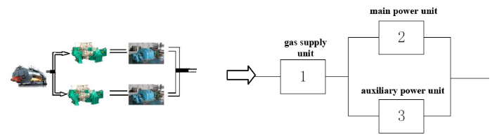
Figure 3.
Structure of a steam turbine power generation system
The components of a steam turbine power generation system can be connected by the reliability block diagram shown in Figure 3. After the research on the inner characteristics of the boiler, steam turbine, and dynamo, we can divide them into multi-state components according to the percentage of normal operating capacity. For gas supply unit 1, the operating capacity is 90% of the designed power and it decreases to 60% during partial deterioration, so the performance vector of gas supply unit 1 is ${{G}_{1}}\in \{{{g}_{11}}=0,{{g}_{12}}=0.6,{{g}_{13}}=0.9\}$. For main power unit 2, the operating capacity can reach 100% of the designed power and it decreases to 60% during partial deterioration, so the performance vector of gas supply unit 1 is ${{G}_{2}}\in \{{{g}_{21}}=0,{{g}_{22}}=0.8,{{g}_{23}}=1.0\}$. The auxiliary power unit 3 is a typical binary-state system, that is, the performance vector is ${{G}_{3}}\in \{{{g}_{31}}=0,{{g}_{32}}=1.0\}$. Suppose the transfer between states of each component is a Markov process of continuous time. Whenthe common cause failure phenomenon is not considered, the component performance parameters are shown in Table 2.
Table 2. Performance parameters of each component in the steam turbine power generation system
| Component | Performance rate | Failure rate | Maintenance rate |
|---|---|---|---|
| 1 | ${{g}_{11}}=0$ | — | $\mu _{12}^{(1)}=120$ |
| ${{g}_{12}}=0.6$ | $\lambda _{21}^{(1)}=0.8$ | $\mu _{23}^{(1)}=150$ | |
| ${{g}_{13}}=0.9$ | $\lambda _{32}^{(1)}=1$ | — | |
| 2 | ${{g}_{21}}=0$ | — | $\mu _{12}^{(2)}=100$ |
| ${{g}_{22}}=0.8$ | $\lambda _{21}^{(2)}=1.5$ | $\mu _{23}^{(2)}=120$ | |
| ${{g}_{23}}=1.0$ | $\lambda _{32}^{(2)}=2$ | — | |
| 3 | ${{g}_{31}}=0$ | — | $\mu _{12}^{(3)}=100$ |
| ${{g}_{32}}=1.0$ | $\lambda _{21}^{(3)}=0.3$ | — |
Because the transition times between different states of each component are subject to exponential distribution, as shown in Figure 4, we can set up differential equations of the probability of every state of each component at time t according to the Kolmogorov equation in the Markov process.
Figure 4.
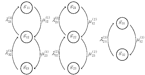
Figure 4.
Transfer relationship between performance rate of each component
For components 1 and 2, namely when $i=1, 2$,
$\left\{ \begin{matrix} & \frac{\text{d}{{p}_{i1}}(t)}{\text{d}t}=\lambda _{21}^{(i)}{{p}_{i2}}(t)-\mu _{12}^{(i)}{{p}_{i1}}(t) \\ & \frac{\text{d}{{p}_{i2}}(t)}{\text{d}t}=\lambda _{32}^{(i)}{{p}_{i3}}(t)-(\lambda _{21}^{(i)}+\mu _{23}^{(3)}){{p}_{i2}}(t)+\mu _{12}^{(3)}{{p}_{i1}}(t) \\ & \frac{\text{d}{{p}_{i3}}(t)}{\text{d}t}=\mu _{23}^{(i)}{{p}_{i2}}(t)-\lambda _{32}^{(i)}{{p}_{i3}}(t) \\ & {{p}_{i1}}(t)+{{p}_{i2}}(t)+{{p}_{i3}}(t)=1 \\ \end{matrix} \right.$
Suppose at the initial time $t=0$, ${{p}_{i1}}(0)=0$, ${{p}_{i2}}(0)=0$, and ${{p}_{i3}}(0)=1$. After MATLAB programming, we can obtain ${{p}_{i1}}(t)$,${{p}_{i2}}(t)$, and ${{p}_{i3}}(t)$, where $i=1, 2$. For component 3, because it is a typical binary system containing only two states, according to Kolmogorov equation:
$\left\{ \begin{matrix} & \frac{\text{d}{{p}_{31}}(t)}{\text{d}t}=\lambda _{21}^{(3)}{{p}_{32}}(t)-\mu _{12}^{(3)}{{p}_{31}}(t) \\ & \frac{\text{d}{{p}_{32}}(t)}{\text{d}t}=\mu _{12}^{(3)}{{p}_{31}}(t)-\lambda _{21}^{(3)}{{p}_{32}}(t) \\ & {{p}_{31}}(t)+{{p}_{32}}(t)=1 \\ \end{matrix} \right.$
Suppose at $t=0$,${{p}_{31}}(0)=0$ and ${{p}_{32}}(0)=1$, then we can also obtain ${{p}_{31}}(t)$ and ${{p}_{32}}(t)$by means of MATLAB programming.According to Equation (1), the universal generating functions of each component are respectively.
${{u}_{1}}(z)=\sum\limits_{{{j}_{1}}=1}^{3}{{{p}_{1{{j}_{1}}}}(t)\cdot {{z}^{{{g}_{1{{j}_{1}}}}}}}={{p}_{11}}(t)+{{p}_{12}}(t)\cdot {{z}^{0.6}}+{{p}_{13}}(t)\cdot {{z}^{0.9}}$
${{u}_{2}}(z)=\sum\limits_{{{j}_{2}}=1}^{3}{{{p}_{2{{j}_{2}}}}(t)\cdot {{z}^{{{g}_{2{{j}_{2}}}}}}}={{p}_{21}}(t)+{{p}_{22}}(t)\cdot {{z}^{0.8}}+{{p}_{23}}(t)\cdot {{z}^{1}}$
${{u}_{3}}(z)=\sum\limits_{{{j}_{3}}=1}^{2}{{{p}_{3{{j}_{3}}}}(t)\cdot {{z}^{{{g}_{3{{j}_{3}}}}}}}={{p}_{31}}(t)+{{p}_{32}}(t)\cdot {{z}^{1}}$
According to Equation (2), the universal generating function of the steam turbine power generation system is
$u(z)=\sum\limits_{{{j}_{1}}=1}^{3}{\sum\limits_{{{j}_{2}}=1}^{3}{\sum\limits_{{{j}_{3}}=1}^{2}{{{p}_{1{{j}_{1}}}}(t){{p}_{2{{j}_{2}}}}(t){{p}_{3{{j}_{3}}}}(t)\cdot {{z}^{f({{g}_{1{{j}_{1}}}},{{g}_{2{{j}_{2}}}},{{g}_{3{{j}_{3}}}})}}}}}$
From the system’s universal generating function, we can determine that there are $3\times 3\times 2=18$ states in total. They are $f({{g}_{11}},{{g}_{21}},{{g}_{31}}),$$f({{g}_{11}},{{g}_{21}},{{g}_{32}}),$$f({{g}_{11}},{{g}_{22}},{{g}_{31}}),$$f({{g}_{11}},{{g}_{22}},{{g}_{32}}),$$f({{g}_{11}},{{g}_{23}},{{g}_{31}}),$$f({{g}_{11}},{{g}_{23}},{{g}_{32}}),$$f({{g}_{12}},{{g}_{21}},{{g}_{31}}),$$f({{g}_{12}},{{g}_{21}},{{g}_{32}}),$$f({{g}_{12}},{{g}_{22}},{{g}_{31}}),$$f({{g}_{12}},{{g}_{22}},{{g}_{32}}),$$f({{g}_{12}},{{g}_{23}},{{g}_{31}}),$$f({{g}_{12}},{{g}_{23}},{{g}_{32}}),$$f({{g}_{13}},{{g}_{21}},{{g}_{31}}),$$f({{g}_{13}},{{g}_{21}},{{g}_{32}}),$$f({{g}_{13}},{{g}_{22}},{{g}_{31}}),$$f({{g}_{13}},{{g}_{22}},{{g}_{32}}),$$f({{g}_{13}},{{g}_{23}},{{g}_{31}}),$ and $f({{g}_{13}},{{g}_{23}},{{g}_{32}}).$
Let ${{G}_{1}}\in \{{{g}_{11}},{{g}_{12}},{{g}_{13}}\},$${{G}_{2}}\in \{{{g}_{21}},{{g}_{22}},{{g}_{23}}\},$ and ${{G}_{3}}\in \{{{g}_{31}},{{g}_{32}}\},$ then the system performance can be represented as ${{G}_{s}}=f({{G}_{1}},{{G}_{2}},{{G}_{3}})$ uniformly. When the system demand $w=0.85$, we can obtain the change of availability, mean output performance, and output performance deficiency of the steam turbine power generation system according to Equations (9) to (16). As the connection structures of components are unknown, when synthesizing system performance, we can assume the system presents different performance characteristics and then calculate reliability indices according to Table 1 and the equations above. When the steam turbine power generation system is regarded as a flow transmission, a task processing MSS, a fixed-weight MSS, and a variable-weight MSS respectively, we find that reliability indices change with time, as shown in Figures 5 to 7.
Figure 5.
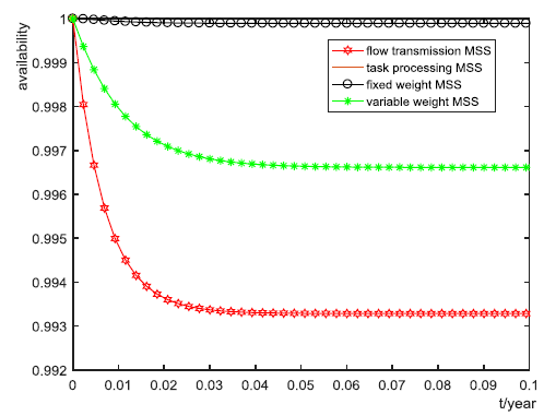
Figure 5.
Availability of MSS
Figure 6.
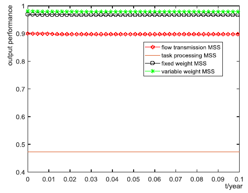
Figure 6.
Mean output performance of MSS
Figure 7.
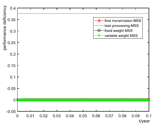
Figure 7.
Mean performance deficiency of MSS
From Figure 5, we can see that the system availability $A(t, w)$ will reach a steady value at about $t=15$ days. When the performance relationships between components can be regarded as flow transmission, the stable availability of the whole system is 0.9933, and when the relationships can be regarded as task processing, the stable availability is 0. When the system performance is calculated by fixed weight UGF, as shown in 3.2, the stable availability is 0.9998; when the system performance is calculated by variable weight UGF, as shown in 3.2, the stable availability is 0.9966. Obviously, only when the steam turbine power generation system is regarded as a task processing MSS will a large deviation appear in the system availability. When the system is regarded as a variable weight MSS, reliability indices are most consistent with the system characteristic itself, and then we can evaluate and optimize reliability parameters of the steam turbine power generation system. Similarly, for system mean output performance and mean performance deficiency, the stable values are shown in Table 3.
Table 3. Steady-state reliability indices values
| Reliability indices System style | Stable availability | Stable output performance | Stable performance deficiency |
|---|---|---|---|
| Flow transmission MSS | 0.9933 | 0.8980 | 0.0017 |
| Task processing MSS | 0 | 0.4730 | 0.3770 |
| Fixed weight MSS | 0.9998 | 0.9675 | $1.8489\times {{10}^{-6}}$ |
| Variable weight MSS | 0.9966 | 0.9742 | $4.1884\times {{10}^{-4}}$ |
From the above analysis, we can determine that when the connection relationship between components is unknown or the performance of the system is uncertain in an MSS, regardless of whether flow transmission or task processing is assumed, the system reliability will be unavoidably disturbed. The method of weighted UGF can deal with the reliability evaluation of uncertain MSSs to a certain extent. For this steam turbine power generation system, variable UGF can reach a better application effect, which is significant to the formulation of maintenance strategies.
5. Conclusions
The universal generating function is an important method for reliability evaluation and optimization of MSSs [25]. On the basis of UGF, aiming at uncertain systems or systems with unknown connection structures, this paper uses OWA operators to weight component performance, designs fixed weight UGF and variable weight UGF, and then synthesizes system output performance. After the comparison of output performance and system demand [26], three reliability evaluation parameters such as availability, mean output performance, and mean performance deficiency are defined. In the case study part, for an uncertain steam turbine power generation system with unknown component connection relationships, we first assume that its functional characteristics are flow transmission MSS and task processing MSS. By comparing and analyzing the proposed methods and existing methods, it is proven that the weighted universal generating function is scientific in the reliability evaluation of uncertain MSSs.
When synthesizing component performance, there are many ways to confirm weight [27]. On the basis of predecessors’ research, this paper makes a reasonable empowerment of component performance through fixed weight and variable weightand obtains satisfactory results. In fact, when applying weighted UGF to the reliability evaluation of MSSs, the weight of each component’s performance has a great influence on system reliability. Therefore, in engineering practice, the rational distribution of weight should be carried out according to the performance relationship between components in MSSs.
Acknowledgements
The authors would like to express their sincere appreciation for the reviewers for their useful suggestions to improve this paper. In addition, this work is supported by the National Natural Science Foundation of China (No. 71671091) and the China Postdoctoral Science Foundation (No. 2018M630561).
Reference
“Preventive Maintenance of Multistate Systems Subject to Shocks, ”
DOI:10.1002/asmb.2151
URL
[Cited within: 1]

Abstract A new approach to optimal maintenance of multistate systems (networks) with binary components is developed. Univariate and multivariate signatures are used for description of system's structure and for efficient dealing with corresponding optimal maintenance problems. A system is subject to a shock process. Each shock destroys in a random way one of the operating components. The first strategy is to perform the preventive maintenance after the system enters one of the intermediate states between the initial UP state and the final absorbing DOWN state. The second strategy is to carry out preventive maintenance after the system experiences k shocks. Some illustrations and numerical results are presented. Copyright 2015 John Wiley & Sons, Ltd.
“The Universal Generating Function in Reliability Analysis and Optimization, ”
DOI:10.1007/1-84628-245-4
[Cited within: 1]

Many real-world systems in engineering are composed of multi-state components that have different performance levels and several failure modes. These have effects on the entire system s performance. §Most books on reliability theory are devoted to traditional binary models that only allow a system either to function perfectly or fail completely. §The Universal Generating Function in Reliability Analysis and Optimization is the first book that gives a comprehensive description of the universal generating function technique and its applications in both binary and multi-state system reliability analysis. §Features:§an introduction to the basic tools used in multi-state system reliability and optimisation;§applications of the universal generating function in the most widely used multi-state systems;§several examples of how the universal generating function can be adapted to different systems in mechanical, industrial and software engineering§The Universal Generating Function in Reliability Analysis and Optimization will be of value to all those interested in multi-state systems in industrial, electrical and nuclear engineering.Many real systems are composed of multi-state components with different performance levels and several failure modes. These affect the whole system's performance.§Most books on reliability theory cover binary models that allow a system only to function perfectly or fail completely.§"The Universal Generating Function in Reliability Analysis and Optimization" is the first book that gives a comprehensive description of the universal generating function technique and its applications in binary and multi-state system reliability analysis.§Features:- an introduction to basic tools of multi-state system reliability and optimization;- applications of the universal generating function in widely used multi-state systems;- examples of the adaptation of the universal generating function to different systems in mechanical, industrial and software engineering.§This monograph will be of value to anyone interested in system reliability, performance analysis and optimization in industrial, electrical and nuclear engineering.Many real-world systems in engineering are composed of multi-state components that have different performance levels and several failure modes. These have effects on the entire system s performance.§Most books on reliability theory are devoted to traditional binary models that only allow a system either to function perfectly or fail completely.§The Universal Generating Function in Reliability Analysis and Optimization is the first book that gives a comprehensive description of the universal generating function technique and its applications in both binary and multi-state system reliability analysis.§Features:§an introduction to the basic tools used in multi-state system reliability and optimization; §applications of the universal generating function in the most widely used multi-state systems; §several examples of how the universal generating function can be adapted to different systems in mechanical, industrial and software engineering. §The Universal Generating Function in Reliability Analysis and Optimization will be of value to all those interested in multi-state systems in industrial, electrical and nuclear engineering. §The Springer Series in Reliability Engineering publishes high-quality books in important areas of current theoretical research and development in reliability, and in areas that bridge the gap between theory and application in areas of interest to practitioners in industry, laboratories, business, and government.
“Multi-State System Reliability Analysis and Optimization for Engineers and Industrial Managers, ”
DOI:10.1007/978-1-84996-320-6
URL
Multi-state System Reliability Analysis and Optimization for Engineers and Industrial Managers presents a comprehensive, up-to-date description of multi-state system (MSS) reliability as a natural extension of classical binary-state reliability. It presents all essential theoretical achievements in the field, but is also practically oriented.New theoretical issues are described, including:* combined Markov and semi-Markov processes methods, and universal generating function techniques;* statistical data processing for MSSs;* reliability analysis of aging MSSs;* methods for cost-reliability and cost-availability analysis of MSSs; and* main definitions and concepts of fuzzy MSS.Multi-state System Reliability Analysis and Optimization for Engineers and Industrial Managers also discusses life cycle cost analysis and practical optimal decision making for real world MSSs. Numerous examples are included in each section in order to illustrate mathematical tools. Besides these examples, real world MSSs (such as power generating and transmission systems, air-conditioning systems, production systems, etc.) are considered as case studies.Multi-state System Reliability Analysis and Optimization for Engineers and Industrial Managers also describes basic concepts of MSS, MSS reliability measures and tools for MSS reliability assessment and optimization. It is a self-contained study resource and does not require prior knowledge from its readers, making the book attractive for researchers as well as for practical engineers and industrial managers.
“Reliability Analysis of Mobile Ad Hoc Networks using Universal Generating Function, ”
DOI:10.1002/qre.1731
URL
[Cited within: 1]
The proliferation of the wireless network over the last decade is one of the significant drivers for the increased deployment of mobile ad hoc networks (MANETs) in the battle field. It is not practically possible to build a fixed wired network infrastructure in battle field. But it is possible to create a mobile wireless network infrastructure because of the mobility of the soldiers. MANET is justified by the possibility of building a network where no infrastructure exists. MANET with group communication applications and multicasting can highly benefit from a networking environment such as military and emergency uses. In such applications, the used ad hoc networks need to be reliable and secure. In recent years, a specific technique called the universal generating function technique (UGFT) has been applied to determine the network reliability. The UGFT is based on an approach that is closely connected to generating functions that are widely used in probability theory. This work devotes to assess the MANET reliability using the UGFT. Reliability of the MANET is defined as the probability that the transformed message from the source can be passed successfully through the MANET and reached the target without any delay. Two kinds of UGFs are discussed in this work, and an algorithm has been proposed to execute the system reliability. This UGFT is illustrated with a case study in a battlefield environment. Copyright 2014 John Wiley & Sons, Ltd.
“Coherent Systems with Multi-State Components, ”
“A Universal Generating Function Approach for the Analysis of Multi-State Systems with Dependent Elements, ”
DOI:10.1016/j.ress.2003.12.002
URL
The paper extends the universal generating function technique used for the analysis of multi-state systems to the case when the performance distributions of some elements depend on states of another element or group of elements.
“A New Approach to Evaluate Reliability of Multistate Networks under the Cost Constraint, ”
DOI:10.1016/j.omega.2004.04.005
URL
[Cited within: 1]
A multistate network is a system composed of multistate components. The network reliability under the cost constraint for level ( d, c) can be computed in terms of ( d, c)-MP (MP stands for minimal path) which is a vector such that d units of flow can be transmitted between two specified nodes with the total cost not greater than c. In this study, a new algorithm was developed to evaluate the reliability of multistate networks under cost constraint in terms of the entire ( d, c)-MPs. The proposed method is more efficient than the best-known existing algorithm. One example is illustrated to show how all ( d, c)-MPs are generated by the proposed algorithm. The reliability of this example is then computed. The computational complexity of the proposed algorithm is also analyzed.
“Extended Block Diagram Method for a Multi-State System Reliability Assessment, ”
“The Markov Reward Model for a Multi-State System Reliability Assessment with Variable Demand, ”
DOI:10.1080/16843703.2007.11673150
URL
[Cited within: 1]
This paper considers reliability measures for a multi-state system where the system and its components can have different performance levels ranging from perfect functioning to complete failure. The suggested approach presents a generalized reliability measure as a functional of trajectories of two stochastic processes output performance of the entire multi-state system and the corresponding demand. It shows how the commonly used reliability measures 120 can be derived from this functional and how they can be computed by using the developed Markov reward model. Corresponding procedures for rewards definition are suggested for different reliability measures. A numerical example is presented in order to illustrate the approach.
“Fuzzy Multi-State Systems: General Definitions, and Performance Assessment, ”
“Interval-Valued Reliability Analysis of Multi-State Systems, ”
DOI:10.1109/TR.2010.2103670
URL
In previous studies that analyzed the reliability of multi-state systems, the precise values of the state performance levels and state probabilities of multi-state components were required. In many cases, however, there are insufficient data to obtain the state probabilities of components precisely. A method is proposed in this paper to analyze the reliability of multi-state systems when the available data of components are insufficient. Based on the Bayesian approach and the imprecise Dirichlet model, the interval-valued state probabilities of components are obtained instead of precise values. The interval universal generating function is developed, and the corresponding operators are defined to estimate the interval-valued reliability of multi-state systems. Affine arithmetic is used to improve the interval-valued reliability. A numerical example illustrates the proposed method. The results show that the proposed method is efficient when state performance levels and/or state probabilities of components are uncertain and/or imprecise.
“Random Fuzzy Extension of the Universal Generating Function Approach for the Reliability Assessment of Multi-State Systems under Aleatory and Epistemic Uncertainties, ”
“A Multi-State Model for the Reliability Assessment of aDistributed Generation System via Universal Generating Function, ”
DOI:10.1016/j.ress.2012.04.008
URL
[Cited within: 1]
The current and future developments of electric power systems are pushing the boundaries of reliability assessment to consider distribution networks with renewable generators. Given the stochastic features of these elements, most modeling approaches rely on Monte Carlo simulation. The computational costs associated to the simulation approach force to treating mostly small-sized systems, i.e. with a limited number of lumped components of a given renewable technology (e.g. wind or solar, etc.) whose behavior is described by a binary state, working or failed. In this paper, we propose an analytical multi-state modeling approach for the reliability assessment of distributed generation (DG). The approach allows looking to a number of diverse energy generation technologies distributed on the system. Multiple states are used to describe the randomness in the generation units, due to the stochastic nature of the generation sources and of the mechanical degradation/failure behavior of the generation systems. The universal generating function (UGF) technique is used for the individual component multi-state modeling. A multiplication-type composition operator is introduced to combine the UGFs for the mechanical degradation and renewable generation source states into the UGF of the renewable generator power output. The overall multi-state DG system UGF is then constructed and classical reliability indices (e.g. loss of load expectation (LOLE), expected energy not supplied (EENS)) are computed from the DG system generation and load UGFs. An application of the model is shown on a DG system adapted from the IEEE 34 nodes distribution test feeder.
“A Combined Method for Reliability Analysis of Multi-State System of Minor-Repairable Components, ”
“Reliability Analysis of Multi-State Systems based on Improved Universal Generating Function, ”
The universal generating function(UGF)is an important approach to the analysis of the reliability of a multi-state system.By decomposition operators, the expansion of the UGF of a load is obtained, and the reliability of a multi-state system is calculated using the inner product operator and the UGF of strength when the common cause failure is taken into account.Reliability models of a multi-state system are established considering the effect of times of load and multi-loads.The influence of the common cause failure and the times of load on the reliability of a multi-state system is studied by an example.The results show that the reliability of a multi-state system and its components is influenced by the common cause failure and times of load, and system reliability decreases obviously when the times of load increase.When the times of load are designated and a common cause failure exists, the reliability of a multi-state system can be calculated directly by means of the model proposed.
“Some Challenges and Opportunities in Reliability Engineering, ”
DOI:10.1109/TR.2016.2591504
URL
[Cited within: 1]
Today's fast-pace evolving and digitalizing World is posing new challenges to reliability engineering. On the other hand, the continuous advancement of technical knowledge and the increasing capabilities of monitoring and computing offer opportunities for new developments in reliability engineering. In this paper, I reflect on some of these challenges and opportunities in research and application. The underlying perspective taken stands on the following: The belief that the knowledge, information, and data (KID) available for the modeling, computations, and analyses done in reliability engineering is substantially grown and continue to do so; The belief that the technical capabilities for reliability engineering have been significantly advanced; The recognition of the increased complexity of the systems, nowadays more and more made of heterogeneous, highly interconnected elements. In line with this perspective, opportunities and challenges for reliability engineering are discussed in relation to degradation modeling and integration of multistate and physics-based models therein, accelerated degradation testing, component-, system- and fleet-wide prognostics and health management in evolving environments. The paper is not a review, nor a state of the art work, but rather it offers a vision of reflection on reliability engineering, for consideration and discussion by the interested scientific community. It does not pretend to give the unique view, nor to be complete in the subject discussed and the related literature referenced to.
“On Ordered Weighted Averaging Aggregation Operators in Multi-Criteria Decision Making, ”
“Reliability of Multi-State Systems with Common Bus Performance Sharing, ”
DOI:10.1080/0740817X.2010.523770
URL
[Cited within: 1]
This article extends an existing model for performance sharing among the multi-state units. The extended model considers an arbitrary number of units that must satisfy individual random demands. If a unit has a performance that exceeds the demand it can transmit the surplus performance to other units. The amount of transmitted performance is limited by the random capacity of a transmission system. The entire system fails if at least one demand is not satisfied. An algorithm based on the universal generating function technique is suggested to evaluate the system reliability and expected performance deficiency. Analytical and numerical examples are presented.
“Reliability of Multi-State Systems with a Performance Sharing Group of Limited Size, ”
DOI:10.1016/j.ress.2016.09.008
URL
[Cited within: 1]
61A new multi-state system with limited performance sharing mechanism is proposed.61The reliability evaluation algorithm is suggested for the new model.61An optimal dynamic connection is derived for the new system.61The expected unsupplied demand is minimized via optimal connection.
“A Method for Interval-Valued Intuitionistic Fuzzy Multiple Attribute Decision Making with Incomplete Weight Information, ”
“An Overview of Methods for Determining OWA Weights, ”
DOI:10.1002/int.20097
URL
[Cited within: 1]
Abstract The ordered weighted aggregation (OWA) operator has received more and more attention since its appearance. One key point in the OWA operator is to determine its associated weights. In this article, I first briefly review existing main methods for determining the weights associated with the OWA operator, and then, motivated by the idea of normal distribution, I develop a novel practical method for obtaining the OWA weights, which is distinctly different from the existing ones. The method can relieve the influence of unfair arguments on the decision results by weighting these arguments with small values. Some of its desirable properties have also been investigated. 08 2005 Wiley Periodicals, Inc. Int J Int Syst 20: 843–865, 2005.
“A New Method of Giving OWA Weights, ”
“Reliability Analysis of Primary Battery Packs based on the Universal Generating Function Method, ”
“How Combined Performance and Propagation of Failure Dependencies Affect the Reliability of a MSS, ”
“Comparison of Objective Weight Determination Methods in Network Performance Evaluation, ”
DOI:10.3724/SP.J.1087.2009.02624
URL
[Cited within: 1]
The methods of standard deviations, maximizing deviations, entropy weight and their improved methods were applied to solve the objective weight determination problem of multivariate indexes in performance evaluation.It made the weight determination selection more comprehensive.The conflict of the indexes was introduced to take account of the correlation between indexes.The case study was implemented in VOIP network.The samples used to compute weights were obtained by simulation.Six weight computing methods were compared for selecting more objective weight determination method.The results show that Criteria Importance Through Intercriteria Correlation(CRITIC) method can get better objective weights.
