


1. Introduction
Clustering [1] is a basic means of data mining in the current big data era, which has been used in many fields such as pattern recognition, image segmentation, and deep learning. Because traditional data clustering methods have certain limitations in processing data, such as low classification accuracy, low efficiency, and poor feasibility, more and more new clustering algorithms have been proposed, such as spectral clustering [2], kernel clustering [3], and integrated clustering [4]. The AP clustering algorithm proposed by Frey et al. [5] quickly became popular due to its fast and effective treatment.
The AP clustering is an algorithm based on the message passing between data points and mainly analyzes the clustering based on the similarity between samples. The algorithm considers each data point as a potential coalescence and effectively weakens the influence of the original center on the clustering effect. However, with the increase of the current data scale and data type, the process of clustering algorithm involves a large amount of computation, thus determining how to preprocess the initial dataset is particularly critical. It is also important to obtain an accurate similarity since the messages r(i, k) and a(i, k) transmitted between AP clustering data points are calculatedon the basis of similarity. [6] proposed a Map/Reduce AP clustering algorithm (MRAP) implemented in the distributed cloud environment Hadoop. Experiments with the K-means algorithm showed that the algorithm has high accuracy and short processing time. [7] proposed a MapReduce-based Distributed AP Clustering Algorithm (DisAP), which randomly divides data points into similarly sized subsets and performs sparse processing to improve the speed and accuracy of the algorithm. [8] proposed a layered AP clustering algorithm (HAP) for large-scale data. This algorithm can adaptively adjust the bias parameters. Compared with AP clustering and adaptive AP clustering, it can ensure the clustering effect and reduce the time energy consumption of clustering. As the AP clustering process needs multiple iterations to update the attractivity matrix R and the attribution matrix A, the clustering operation is slower. For this reason, [9] proposed a map/reduce AP clustering method based on Hadoop. The algorithm is performed after partitioning the data in the map phase, and the clustering results are merged in the reduce stage. Although the algorithm reduces the clustering iterations of the process, its clustering effect is easily affected by the merging strategy. Therefore, how to improve the operating efficiency of the algorithm while maintaining the original clustering effect is worth considering.
In order to solve the above problems, this paper proposes a coarse-grained parallel AP clustering algorithm based on intra-class and inter-class distance: IOCAP. The algorithm first proposes a coarse-grained partitioning strategy, which roughly divides the original dataset to be clustered into multiple subsets and initially reduces the complexity of the problem. Afterwards, the intra-class and inter-class distances are introduced to calculate the similarity in the AP algorithm, which can improve the accuracy of the clustering algorithm. Finally, the algorithm is arranged on the MapReduce model to achieve the parallelization of the AP clustering and improve the efficiency of the algorithm.
2. Related Work
2.1. Granularity
The granularity is initially used in the data warehouse to represent the data refinement and integration level of the data unit. Grains have different granularity, that is, the size of the grain. The calculation of granularity is mainly to simplify the cognition of things, thus reducing the complexity of problem solving.
According to the refinement standard of data granularity, the higher the degree of refinement, the smaller the granularity. Conversely, the lower the refinement degree, the greater the granularity. In parallel computing, the program needs to be divided according to parallel conditions to obtain parallel equivalent particles of different sizes. In some cases, the calculation can be completed by using a coarser granularity, but in some cases the granularity must be refined [10] before proceeding. The introduction of granularity can reduce the size of clustering data and effectively improve the efficiency of clustering algorithm. However, it is not uniform and unreasonable to divide the program only based on the parallel equivalent particles. With the refinement of the calculation granularity, the total traffic will increase, resulting in greater overhead. Therefore, how to scientifically and reasonably determine the granularity to divide a dataset has become an important issue in current research.
2.2. AP Clustering Algorithm
AP clustering is an algorithm based on message passing between data points. It mainly passes two types of messages: responsibility and availability [11]. The algorithm does not need to set the number of clusters in advance, and the most suitable clustering can be determined based on the communication between the data points.
The AP algorithm performs clustering calculations based on the similarity [12], where characteristics are symmetrical or asymmetrical. Among them, symmetry refers to the similarity between two data points and asymmetry refers to the dissimilarity between two data points. The similarity of s(i, j) is set to the N×N similarity matrix S. The diagonal values on the matrix S are s(k, k); the larger the value is, the more likely it will become the center of the cluster, which is also called the bias parameter p(k)=s(i, i). Introduce the responsibility matrix R=[r(i, k)] and the availability matrix A=[a(i, k)], where r(i, k) is a message that is sent by pointing i to the candidate cluster center k, indicating the degree to which the data point k is suitable as the clustering center of the data point i. a(i,k) is the message that is sent from k to the data point i, indicating the fitness of the data point ifor selecting the data point k as its clustering center. The iterative formula is as follows:
Among Equations (1) and (2), $a(i,{k}')$ represents the recognition (availability) degree of the data point i to the point ${k}'$, and $r({i}',k)$ represents the degree of availability of the data point k to other data points.
The AP algorithm continuously updates the availability and the attribution value of each data point through an iterative process until multiple high-quality cluster centers are generated, and the remaining data points are assigned to the corresponding clusters. Because the vibration is easily generated when parameters are updated in the clustering process, the damping coefficient dampneedsbe introduced to converge:
In Equations (3) and (4),${R}'$and${A}'$ represent the information values for the previous iteration. The value of damp is set between 0 and 1,and it is set to 0.5 in this paper.
3. Coarse-Grained Partitioning Parallel AP Clustering Algorithm based on Intra-Class and Inter-Class Distances
In this section, the coarse-grained partitioning is first introduced to roughly classify clustered datasets, and then it combines intra-class and inter-class distance for similarity calculation to improve the AP clustering algorithm. On this basis, this paper proposes a parallel improved AP clustering algorithm based on MapReduce: IOCAP.
3.1. Coarse-Grained Partitioning Strategy
With the expansion of the scale and type of big data, the ability of data mining processing has become an increasingly prominent problem. The extensive application of parallel clustering technology effectively alleviates the low efficiency of clustering algorithms. In parallel computing, the granularity is used to divide the dataset, and as many parallel particles as possible are found simplify the dataset to improve the efficiency of data processing. However, because many datasets are not parallel to a certain size, it is necessary to divide them in order to find the appropriate size of the particles to form different data subsets of the granularity level, which helps reduce the noise data and makes the dataset have greater parallelism.
This paper divides the data based on the coarse-grained strategy. Set the sample dataset $\text{M}=\{{{m}_{1}},\text{ }{{m}_{2}},\text{ }\cdots ,\text{ }{{m}_{\ell }}\}$, which contains $\ell $ sample objects. The distance(Euclidean distance) between any data is dist(di,dj),and the granularity variable is Gv, which represents the fusion radius of the data origin. The Equation (5) is:
According to Gv, the distance between two sample data is less than Gv, the adjacent data are initiallydivided into multiple sample clusters, and the sample cluster mean(geometric center) avg represents the cluster.For (m1, m2), (m2, m3), and (m3, m4)sample point pairs, calculate the Euclidean distance [13] between every two sample points. If the distance between sample points is less than Gvand these points are distributed adjacently, they can be divided into the same cluster, and the mean avg is used to represent the cluster. The initial cluster centeris selected through different levels of granularity. The dataset is divided based on the coarse-grained strategy aims to preprocess the initial dataset.The selection of coarse-grained particles can effectively avoid the increase of traffic caused by the high granularity of the data unit, thereby improving the efficiency of the AP clustering algorithm.
The steps for dividing a dataset based on a coarse-grained strategy are as follows:
Step 1 The sample points in the sample dataset $\text{M}=\{{{m}_{1}},\text{ }{{m}_{2}},\text{ }\cdots ,\text{ }{{m}_{\ell }}\}$ are stored in an adjacent distance matrixNdm=Nn×Nn, where Nn is the total number of data of the dataset M, and each row of the matrix represents the distance between the data m1 in the dataset M and other data.
Step 2 Initialize the granularity variable Gv.The matrix Nm is divided by the granularity variable Gv, and the fused data are divided into a single sample cluster C={avg1, avg2,
Step 3 Rank the sample clustersrank(AVGi), which areobtained according to the pre-defined size.
Step 4 Observe the ranking results and propose the sample clusters with the highest n granularity levels as the initial clustering of the AP clustering algorithm.
Step 5 Remove noise points with a granularity level of 1 and output new datasets U={u1, u2,
3.2. Coarse-Grain AP Clustering based on Intra-Class and Inter-Class Distances
3.2.1. Intra-Class and Inter-Class Distances
Since the AP algorithm implements clustering mainly through the similarity matrix between sample data, the calculation of the similarity matrix is extremely important and is related to the accuracy of the clustering result. The AP algorithm generally determines the clustering based on the Euclidean metric, which is a typical dissimilarity measure. Its calculation formula is as follows:
In Equation (6), D represents a function D: X×X→R, x, y∈X and where xi, yi represent the ith and jth coordinates of x and y respectively. Although the calculation of Euclidean distance is more intuitive, it does not take into account the random fluctuations that the measurement values may have and the effect of isolated points on the dispersion between classes in the sample data, so there are certain limitations.
In this paper, the intra-class distance and inter-class distance [14] are used to judge the similarity between data points to determine the optimal number of clustering samples and strengthen the clustering effect of the AP algorithm. The dataset U={u1,u2,
In Equation (7), $u_{ik}^{j}$ represents the kth dimension data of the data object uiin the class Tj, and ni represents the total number of data objects in the Tj. The intra-class distance can describe the degree of similarity between data elements within a class, so the smaller the value, the better.
The average distance between the data object xi in the cluster Tj and all classes other than Tj, that is, the inter-class distance, is:
In Equation (8),thk represents the kth dimensional data of data center th in classTh. The inter-class distance E(i, j) represents the average distance between objects in the class and other class objects, so the larger the value, the better.
The similarity that includes the intra-class distance and inter-class distances is calculated as follows:
From Equation (9),when the intra-class distance is small and the class spacing is large, the clustering effect is best when the value IG(i, j) is close to 1, and the clustering effect is poor when the value IG(i, j) is close to -1.
3.2.2. Improved AP Clustering with Coarse-Grained Partitioning
By using intra-class and inter-class distances to construct the similarity between sample data points, the clustering algorithm can simultaneously consider the degree of closeness within sample classes and the degree of dispersion between sample classes. Assuming that there are n data that constitute the similarity matrix of N×N, ${S}'(i,j)$ is the degree of similarity between sample data points i and j, according to Equation (10):
The clustering center can be evaluated by the diagonal element value${S}'(i,j)$of the matrix${S}'.$The clustering effect is optimal when the value of ${S}'(i,j)$ tends to 1.
The coarse-grained AP clustering algorithm based on intra-class and inter-class distances first selects suitable coarse particles to preprocess the original dataset. After fusion, the sample datasets are divided into n subsets. Then, the similarity of data points in each subset is calculated by intra-class and inter-class distances. AP clustering is carried out to generate clustering sets. The specific process is shown in Algorithm 1.
Algorithm 1 Coarse-grained AP clustering algorithm based on intra-class and inter-class distances
Input: Dataset Z={z1, z2,
Output: Clustering result set and clustering center
Step 1 According to the coarse-grained strategy, the dataset is coarsely divided
1. Initialization: Initialize the granularity variable Gv;
2. Save the sample data in the dataset Z into the matrix Ndm;
3. Calculate the variable Gv according to Equation (5), and then subdivide the data that is smaller than Gv and adjacent data to clusters C(avgi);
4. After calculating the mean value avgi, the cluster of data is ranked according to the set coarse particles, and the clusters with the highest k levels are taken out;
5. Get a new dataset;
Step 2 Find the matrix R and A for the divided dataset U
1. Initialization: Let the similarity ${s}'(k,k)$ be the same value and assign it to the parameter p; let r(i,k)=0, a(i,k)=0 and store them in the matrix R and A respectively; Damping coefficient damp=0.5;
2. ${R}'$=R, ${A}'$=A;
3. Take the (t-1) times running results of A and the t iterations of R separately;
4. Calculate R according to the Equation, which represents the similarity calculated from the introduced intra-class and inter-class distances, and calculate A according to Equation (2);
5. When $k={k}',$ calculating r(k, k) according to the formula $r(k,\text{ }k)=p(k)-\max \{a(k,\text{ }{k}')+{s}'(k,\text{ }{k}')\}$ and put it into R and calculating a(k, k) according to Equation (2) and stored in A;
6. R=damp×${R}'$+(1-damp)×R, A=damp×${A}'$+(1-damp)×A;
7. Save the results of the t iterations of R and A respectively;
Step 3 Determine if the iteration end condition is satisfied
1. The clustering center remains stable after multiple iterations of updates;
2. The prescribed number of iteration exceeds the limits;
If one of the above conditions is satisfied, stopping iterating and go to Step 4, otherwise go back to Step 2.
Step 4 Output the final clustering result set and clustering center.
3.3. The Implementation of Improved AP Clustering in MapReduce
After coarse-grained AP clustering based on intra-class and inter-class distances, the MapReduce model [15] was used to optimize the algorithm by parallelizing the improved AP clustering. The IOCAP algorithm mainly includes two MapReduce processes in Figure 1. The first stage is to perform parallel AP clustering on the granularity-divided subsets, including Mapper1 and Reducer1, where Mapper1 acquires n datasets after granularity partitioning and Reducer1 performs AP clustering on n datasets in parallel, resulting in cluster representative and cluster center. The second stage consists of Mapper2 and Reducer2, which use the cluster representation formed in the first stage to indicate the final polycentricity for all data points.
Figure 1
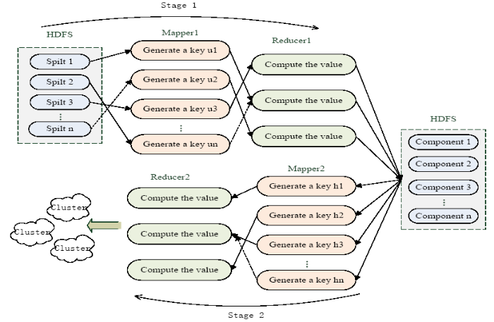
Figure 1.
IOCAP clustering
The MapReduce process corresponding to the IOCAP algorithm is specifically expressed as follows:
Algorithm 2 IOCAP algorithm
Step 1 IOCAP Mapper1 algorithm
Input: Line number key of the dataset U, data unit $value {{u}_{\varepsilon }}$and the amount of data divided n
Output: key-value pair $\text{}ke{y}',\text{ }valu{e}'\text{}$, which $ke{y}'$ represents the cluster’s label, $valu{e}'$ represents the data unit
1. Get data subset U={u1, u2,
2. Let $ke{y}'=\delta, \text{ }valu{e}'={{u}_{\varepsilon }}$, and output data key-value pairs $\text{}ke{y}',\text{ }valu{e}'\text{}$;
Step 2 IOCAP Reducer1 algorithm
Input:Cluster label key, data list vaList which containing the same key value, damping coefficient damp in AP clustering algorithm
Output: HDFS file, where each row represents the clustering representation hi,i =1,2,
1. According to the data list vaList, the similarity matrix ${{{S}'}_{n}}$’ and the bias parameters Pn’ are calculated by using the intra-class and inter-class distances (Equation (10));
2. The AP clustering is carried out through the similarity matrix ${{{S}'}_{n}}$’ and the bias parameter Pn’, and the clustering representation is generated;
3. Store the data units hi∈Hn’,i =1, 2,
Step 3 IOCAP Mapper2 algorithm
Input:Line number key of the dataset U, data unit $ value {{u}_{\varepsilon }}$
Output: key-value pair $\text{}ke{y}',\text{ }valu{e}'\text{}$, where $ke{y}'$ represents the cluster label $Num(\varepsilon )$, $valu{e}'$ represents the data unit ${{u}_{\varepsilon }}$
1. Mapper2 removes the cluster representation Hn’ from the cache;
2. Get the cluster representation Hn’ that is most similar to the data point ${{u}_{\varepsilon }}$in the cluster representative set$Num(\varepsilon )$;
3. Let $key'=Num(\varepsilon ),\text{ }valu{e}'={{u}_{\varepsilon }}$, and output data pairs $\text{}ke{y}',\text{ }valu{e}'\text{}$;
Step 4 IOCAP Reducer2 algorithm
1. Reducer2 summarizes the clustering results and outputs the final cluster and clustering center.
4. Experiments and Analysis
4.1. Experimental Dataset
To verify the impact of the IOCAP algorithm on the clustering effect, experiments are performed using the Iris dataset [16], the Diabetes dataset, and the MNIST (hand written digital) dataset. K-means clustering, the classic AP algorithm, and the IOCAP algorithm are used to cluster three kinds of datasets respectively. The damping coefficient damp of the algorithm is set to 0.5, the maximum number of iterations is set to 1200, the value of the granularity variable Gv is set to 0.6, and the number of iterations that make the centroid remain stable is set to 120 times.
4.2. Evaluation of Clustering Performance
In order to measure the merits of the clustering algorithm, the ACC index [17], the Purity index, and the NMI index are introduced to measure the accuracy of the clustering algorithm.
4.2.1. ACC (Accuracy) Index
Among Equation (11), n represents the number of data points, and ci and ui represent the actual cluster label and the obtained cluster label respectively. $\delta (c,u)$indicates that when c=u, the function value is 1; otherwise, $\delta (c,u)=0.$ The map function maps the obtained cluster tag to the actual tag, and the map can be obtained using the Kuhn-Munkres algorithm [18]. The larger the ACC value, the closer the clustering result is to the actual cluster.
4.2.2. Purity Index
The Purity index is evaluated by calculating the proportion of the correct data in the cluster to the total data.
AmongEquation (12), n represents the number of data points,${{\psi }_{k}}\in \Psi ,k=1,2,\cdots ,\left| \left. \Psi \right| \right.$, and ${{\psi }_{k}}$is the set of the kth cluster.$\Phi =\text{ }\!\!\{\!\!\text{ }{{\phi }_{\text{1}}},\text{ }{{\phi }_{\text{2}}},\text{ }\cdots ,\text{ }{{\phi }_{n}}\text{ }\!\!\}\!\!\text{ }$, and ${{\phi }_{j}}$ is the jth data. Purity∈[0,1], andthe closer the Purity value is to 1, the more accurate the clustering result is.Otherwise, the closer the value is to 0, the higher the error rate clustering.
4.2.3. NMI (Normalized Mutual Information) Index
This indicator is often used to measure the similarity of two clustering. SetU and Vas the distribution of N sample data. The entropy (representing the degree of uncertainty) of the two distributions is shown in Equation (13):
Among them:
In Equation(14), P(i) is the number of data of cluster i, ${P}'(j)$ is the number of data of cluster j, and N represents the total number of data.
The mutual information (MI) between U and V is shown in Equation (15):
Among them:
In Equation(16), P(i, j) is the same number of data in the ith cluster as in the real tag j.
The standardized MI, that is, NMI is shown in Equation(17):
The range of NMI values is [0,1], and the higher the value, the higher the degree of similarity between the two clusters.
4.3. Analysis of Experimental Results
1) The running time of the AP algorithm and the IOCAP algorithm on the three datasetsare calculated. The experimental result data is taken as the average of multiple runs. The details are shown in Table 1:
Table 1. The comparison of the running time of AP algorithm and IOCAP algorithm
| Datasets | Data scale | Number of cluster | AP clustering runtimes/s | IOCAP clustering runtimes/s |
|---|---|---|---|---|
| Iris | 150 | 3 | 0.0260 | 0.0347 |
| Diabetes | 442 | 4 | 0.2076 | 0.3056 |
| MNIST | 5620 | 1797 | 155.2385 | 89.1252 |
From the experimental results, it can be seen that for a smaller dataset, the running time of the IOCAP algorithm is not faster than that of the AP algorithm. However, for large-scale data, the IOCAP algorithm significantly shortens the clustering time and improves the efficiency of the algorithm. This is because the IOCAP algorithm first preprocesses the original dataset, that is, it reduces the data size through coarse-grained partitioning, and then combined with the MapReduce model, the divided subsets are clustered in parallel. Compared with the AP algorithm, the IOCAP algorithm has obvious advantages in the clustering of large datasets. However, for the smaller dataset, as a result of the IOCAP algorithm in data preprocessing, the calculation of the similarity matrix has occupied a certain time. Thisincreases the communication overhead and makes the algorithm efficiency decline.
2) In order to measure the pros and cons of the algorithm, the average ACC index, Purity index, and NMI index of the K-means algorithm, AP algorithm,and IOCAP algorithm on the three datasets are calculated and compared. In the experiment, each algorithm is executed 25 times and the average value of three indicators is taken.
a. Iris dataset
The Iris dataset contains 150 data points and three types, and each data corresponds to a 4-dimensional vector. The clustering performance of the three algorithms is shown in Table 2.
Table 2. Evaluation indexes of three algorithms on the Iris dataset (p is mean)
| K-means | AP | IOCAP | |
|---|---|---|---|
| ACC | 0.8117 | 0.6600 | 0.8425 |
| Purity | 0.8707 | 0.6600 | 0.8770 |
| NMI | 0.7225 | 0.6751 | 0.7800 |
In this experiment, the number of clusters of the K-means algorithm is set to 3. As can be seen from Table 1, each index of the IOCAP algorithm is all improved compared to the AP algorithm on the cluster evaluation indexes ACC, Purity, and NMI. Because the K-means algorithm needs to specify the number of clusters in advance and there are large fluctuations in the clustering process, the algorithm is very unstableand there is a certain limit. Experiments show that the clustering effect of the IOCAP algorithm on the Iris dataset is better.
b. Diabetes dataset
The Diabetes dataset consists of 442 data, which are divided into four types. The clustering performance of the three algorithms is shown in Table 3.
Table 3. Evaluation indexes of three algorithms on the Diabetes dataset (p is mean)
| K-means | AP | IOCAP | |
|---|---|---|---|
| ACC | 0.4710 | 0.0845 | 0.4920 |
| Purity | 0.6898 | 0.1082 | 0.8962 |
| NMI | 0.0091 | 0.1514 | 0.0112 |
In this experiment, the number of clusters of the K-means algorithm is set to 2. From Table 2, it can be seen that the IOCAP algorithm performs better on the ACC and purity indicators, but it is inferior to the AP algorithm on the NMI indicator. Compared with the K-means algorithm and AP algorithm, the IOCAP algorithm occupies a certain advantage.
c. MNIST dataset
The MNIST dataset contains 5620 hand-written digital data. The clustering performance of the three algorithms is shown in Table 4.
Table 4. Evaluation Indexes of three algorithms on the MNIST dataset (p is mean)
| K-means | AP | IOCAP | |
|---|---|---|---|
| ACC | 0.6090 | 0.2122 | 0.8094 |
| Purity | 0.8078 | 0.2118 | 0.8925 |
| NMI | 0.6051 | 0.6088 | 0.8295 |
In this experiment, the number of clusters of the K-means algorithm is set to 40. From Table 4, it can be seen that the AP algorithm performs poorly on this dataset on a relatively large dataset, and the K-means algorithm performs relatively well. But the IOCAP algorithm is superior to other indicators. This shows that IOCAP algorithm has better clustering performance for large-scale datasets.
Through three comparison experiments and the combination of three evaluation indicators, the IOCAP algorithm is superior to the K-means algorithm and the AP algorithm as a whole. This shows that the algorithm guarantees the clustering efficiency to some extent and also improves the accuracy. Therefore, considering the time, accuracy, and communication overhead of clustering, the advantages of IOCAP are obvious, and it is also more suitable for efficient and accurate clustering of large datasets.
5. Conclusion
For the current high-dimensional and complex data processing in the era of big data, the classic AP clustering algorithm has been difficult to meet its needs. The IOCAP algorithm uses a coarse-grained idea to simplify the dataset initially and then improves the AP clustering algorithm by combining the concepts of intra-class and inter-class distances, which greatly improves the accuracy of the algorithm. A parallelized improved AP algorithm based on the MapReduce modelis then implemented. Later, the improved AP algorithm based on the MapReduce model to achieve parallelization improves the algorithm's ability to handle large-scale data and clustering efficiency. For the clustering of complex large datasets, the advantages of the IOCAP algorithm can be clearly seen. The next step is to explore the issue of how to optimize the granularity of parallel particles and the speedup of clustering operations when the structure and time-space relationship of big data arecomplex.
Acknowledgement
This work was partly financially supported through grants from the National Natural Science Foundation of China (No.61672470) andthe Open Issues of Beijing CityKey Laboratory (No.BKBD-2017KF08).
Reference
P-PIC: Parallel Power Iteration Clustering for Big Data
,”
DOI:10.1016/j.jpdc.2012.06.009
URL
[Cited within: 1]

78 Proposed parallel power iteration clustering algorithm. 78 Implemented the p-PIC algorithm using MPI. 78 Ran the p-PIC algorithm on different data sizes. 78 Ran the algorithm on both cluster and cloud computers. 78 Obtained almost linear speedups.
Cluster Ensemble based on Spectral Clustering
,”
Towards Hybrid Clustering Approach to Data Classification: Multiple Kernels based Interval-Valued Fuzzy C-Means Algorithms
,”
DOI:10.1016/j.fss.2015.01.020
URL
[Cited within: 1]

In this study, kernel interval-valued Fuzzy C-Means clustering (KIFCM) and multiple kernel interval-valued Fuzzy C-Means clustering (MKIFCM) are proposed. The KIFCM algorithm is built on a basis of the kernel learning method and the interval-valued fuzzy sets with intent to overcome some drawbacks existing in the onventional Fuzzy C-Means (FCM) algorithm. The development of the method is motivated by two factors. First, uncertainty is inherent in clustering problems due to some information deficiency, which might be incomplete, imprecise, fragmentary, not fully reliable, vague, contradictory, etc. With this regard, interval-valued fuzzy sets exhibit advantages when handling such aspects of uncertainty. Second, kernel methods form a new class of pattern analysis algorithms which can cope with general types of data and detect general types of relations (geometric properties) by embedding input data in a vector space based on the inner products and looking for linear relations in the space. However, as the clustering problems may involve various input features exhibiting different impacts on the obtained results, we introduce a new MKIFCM algorithm, which uses a combination of different kernels (giving rise to a concept of a composite kernel). The composite kernel was built by mapping each input feature onto individual kernel space and linearly combining these kernels with the optimized weights of the corresponding kernel. The experiments were completed for several well-known datasets, land cover classification from multi-spectral satellite image and Multiplex Fluorescent In Situ Hybridization (MFISH) classification problem. The obtained results demonstrate the advantages of the proposed algorithms.
A Feature Grouping Method for Ensemble Clustering of High-Dimensional Genomic Big Data
,” in
DOI:10.1109/FTC.2016.7821620
URL
[Cited within: 1]
High-dimensional genomic big data with hundred of features present a big challenge in cluster analysis. Usually, genomic data are noisy and have correlation among the features. Also, different subspaces exist in high-dimensional genomic data. This paper presents a feature selecting and grouping method for ensemble clustering of high-dimensional genomic data. Two most popular clustering methods: k-means and similarity-based clustering are used for ensemble clustering. Ensemble clustering is more effective in clustering high-dimensional complex data than the traditional clustering algorithms. In this paper, we cluster un-labeled genomic data (148 Exome data sets) of Brugada syndrome from the Centre of Medical Genetics, VUB UZ Brussel using SimpleKMeans, XMeans, DBScan, and MakeDensityBasedCluster algorithms and compare the clustering results with proposed ensemble clustering method. Furthermore, we use biclustering ( -Biclustering) algorithm on each cluster to find the sub-matrices in the genomic data, which clusters both instances and features simultaneously.
Clustering by Passing Messages Between Data Points
,”
DOI:10.1126/science.1136800
URL
PMID:17218491
[Cited within: 1]
Clustering data by identifying a subset of representative examples is important for processing sensory signals and detecting patterns in data. Such "exemplars" can be found by randomly choosing an initial subset of data points and then iteratively refining it, but this works well only if that initial choice is close to a good solution. We devised a method called "affinity propagation," which takes as input measures of similarity between pairs of data points. Real-valued messages are exchanged between data points until a high-quality set of exemplars and corresponding clusters gradually emerges. We used affinity propagation to cluster images of faces, detect genes in microarray data, identify representative sentences in this manuscript, and identify cities that are efficiently accessed by airline travel. Affinity propagation found clusters with much lower error than other methods, and it did so in less than one-hundredth the amount of time.
Map/Reduce Affinity Propagation Clustering Algorithm
,”
Distributed Affinity Propagation Clustering based on MapReduce
,”
Hierarchical Affinity Propagation Clustering for Large-Scale Dataset
,”Affinity Propagation(AP)has advantages on efficiency and accuracy,and has no need to set the number of clusters,but is not suitable for large-scale data clustering.Hierarchical Affinity Propagation(HAP)was proposed to overcome this problem.Firstly,the data set was divided into several subsets that can be effectively clustered by AP to select the exemplars of each subset.Then,AP clustering was implemented again on all the subset exemplars to select exemplars of the whole data set.Finally,all the data points were clustered according to similarities with the exemplars,and realizing efficient clustering of large-scale data set.The experimental results on real and simulated data sets show that, compared with traditional AP and adaptive AP,HAP reduces the time consumption greatly and achieves a good clustering result in the meanwhile.
Map/Reduce Affinity Propagation Clustering Algorithm
,” in
The Elephant and the Mice:The Role of Non-Strict Fine-Grain Synchronization for Modern Many-Core Architectures
”in
DOI:10.1145/1995896.1995948
URL
[Cited within: 1]
The Cray XMT architecture has incited curiosity among computer architect and system software designers for its architecture support of fine-grain in-memory synchronization. Although such discussion go back thirty years, there is a lack of practical experimental platforms that can evaluate major technological trends, such as fine-grain in-memory synchronization. The need for these platforms becomes apparent when dealing with new massive many-core designs and applications. This paper studies the feasibility, usefulness and trade-offs of fine-grain in-memory synchronization support in a real-world large-scale many-core chip (IBM Cyclops-64). We extended the original Cyclops-64 architecture design at gate level to support the fine-grain in-memory synchronization feature. We performed an in-depth study of a well-known kernel code: the wavefront computation. Several versions of the kernel were used to test the effects of different synchronization constructs using our chip emulation framework. Furthermore, we tested selected OpenMP kernel loops against existing software-based synchronization approaches. In our wavefront benchmark study, the combination of fine-grain dataflow-like in-memory synchronization with non-strict scheduling methods yields a thirty percent improvement over the best optimized traditional synchronization method provided by the original Cyclops-64 design. For the OpenMP kernel loops, we achieved speeds of three to fourteen times the speed of software-based synchronization methods.
Adaptive Noise Immune Cluster Ensemble Using Affinity Propagation
,” in
DOI:10.1109/TKDE.2015.2453162
URL
[Cited within: 1]
Cluster ensemble, as one of the important research directions in the ensemble learning area, is gaining more and more attention, due to its powerful capability to integrate multiple clustering solutions and provide a more accurate, stable and robust result. Cluster ensemble has a lot of useful applications in a large number of areas. Although most of traditional cluster ensemble approaches obtain good results, few of them consider how to achieve good performance for noisy datasets. Some noisy datasets have a number of noisy attributes which may degrade the performance of conventional cluster ensemble approaches. Some noisy datasets which contain noisy samples will affect the final results. Other noisy datasets may be sensitive to distance functions.
Data Stream Clustering with Affinity Propagation
,”
DOI:10.1109/TKDE.2013.146
URL
[Cited within: 1]
Data stream clustering provides insights into the underlying patterns of data flows. This paper focuses on selecting the best representatives from clusters of streaming data. There are two main challenges: how to cluster with the best representatives and how to handle the evolving patterns that are important characteristics of streaming data with dynamic distributions. We employ the Affinity Propagation (AP) algorithm presented in 2007 by Frey and Dueck for the first challenge, as it offers good guarantees of clustering optimality for selecting exemplars. The second challenging problem is solved by change detection. The presented StrAP algorithm combines AP with a statistical change point detection test; the clustering model is rebuilt whenever the test detects a change in the underlying data distribution. Besides the validation on two benchmark data sets, the presented algorithm is validated on a real-world application, monitoring the data flow of jobs submitted to the EGEE grid.
An Enhanced Support Vector Machine Classification Framework by Using Euclidean Distance Function for Text Document Categorization
,”
PossibilisticClustering Segmentation Algorithm based on Intra-Class and Inter-Class Distance
,”Objective As image segmentation technology has continued to develop,scholars have proposed numerous algorithms for image segmentation. Image complexity and structure instability have resulted in a growing number of image segmentation methods,which provide segmentation effects for different types of images. To further improve noise immunity and the accuracy of image segmentation,an improved possibilistic clustering algorithm combining intra-class distance and interclass distance is proposed and applied to image segmentation. Method The algorithm uses a possible measure to describe the degree of membership. The constraint that memberships of sample points across clusters must sum to 1 in fuzzy c-means is removed using a possibility measure so that membership degree is suitable for the characterization of"typical"and"compatibility". The algorithm avoids the traditional possibilistic clustering segmentation algorithm that only considers the dis-tance of the sample to the cluster center. In this paper,intra-class and inter-class distances are combined as a new measure for the algorithm,with consideration of both the intra-class compactness and the inter-class scatter degree,to improve the stability and anti-noise ability of different clustering structures. The histogram is integrated into the possibility of the fuzzy clustering segmentation algorithm so that it can achieve segmentation of all types of complex images. Result Through synthetic and remote sensing images,segmentation tests show that the proposed improved possibilistic clustering algorithm is effective,segmentation contour is clear,and classification accuracy and noise are small. Compared with other algorithms,the error rate is reduced by 2 percentage points,and the result is more satisfactory. Conclusion This study aims to conduct fuzzy c-means clustering segmentation algorithm and possibilistic clustering segmentation algorithm for image classification with similar backgrounds and targeting color inaccuracy defects by combining intra-class distance and inter-class distance as measures of the algorithm effectively to solve the image segmentation problem classification. This method,combined with the histogram,is proposed for a fast possibilistic fuzzy clustering segmentation algorithm that is also applicable for complex,large images.
Optimized Big Data K-means Clustering using MapReduce
,”
DOI:10.1007/s11227-014-1225-7
URL
[Cited within: 1]
Clustering analysis is one of the most commonly used data processing algorithms. Over half a century, K-means remains the most popular clustering algorithm because of its simplicity. Recently, as data volume continues to rise, some researchers turn to MapReduce to get high performance. However, MapReduce is unsuitable for iterated algorithms owing to repeated times of restarting jobs, big data reading and shuffling. In this paper, we address the problems of processing large-scale data using K-means clustering algorithm and propose a novel processing model in MapReduce to eliminate the iteration dependence and obtain high performance. We analyze and implement our idea. Extensive experiments on our cluster demonstrate that our proposed methods are efficient, robust and scalable.
Online Active Learning of Decision Trees with Evidential Data
,”
DOI:10.1016/j.patcog.2015.10.014
URL
[Cited within: 1]
61Active belief decision trees are learned from uncertain data modelled by belief functions.61A query strategy is proposed to query the most valuable uncertain instances while learning decision trees.61To deal with evidential data, entropy intervals are extracted from the evidential likelihood.61Experiments with UCI data illustrate the robustness of proposed approach to various kinds of uncertain data.
Parallel Spectral Clustering in Distributed Systems
,”
DOI:10.1109/TPAMI.2010.88
URL
PMID:20421667
[Cited within: 1]
Spectral clustering algorithms have been shown to be more effective in finding clusters than some traditional algorithms, such as k-means. However, spectral clustering suffers from a scalability problem in both memory use and computational time when the size of a data set is large. To perform clustering on large data sets, we investigate two representative ways of approximating the dense similarity matrix. We compare one approach by sparsifying the matrix with another by the Nystro m method. We then pick the strategy of sparsifying the matrix via retaining nearest neighbors and investigate its parallelization. We parallelize both memory use and computation on distributed computers. Through an empirical study on a document data set of 193,844 instances and a photo data set of 2,121,863, we show that our parallel algorithm can effectively handle large problems.
Kuhn-Munkres Parallel Genetic Algorithm for the Set Cover Problem and its Application to Large-Scale Wireless Sensor Networks
,”
DOI:10.1109/TEVC.2015.2511142
URL
[Cited within: 1]
Operating mode scheduling is crucial for the lifetime of wireless sensor networks (WSNs). However, the growing scale of networks has made such a scheduling problem more challenging, as existing set cover and evolutionary algorithms become unable to provide satisfactory efficiency due to the curse of dimensionality. In this paper, a Kuhn-Munkres (KM) parallel genetic algorithm is developed to solve the set cover problem and is applied to the lifetime maximization of large-scale WSNs. The proposed algorithm schedules the sensors into a number of disjoint complete cover sets and activates them in batch for energy conservation. It uses a divide-and-conquer strategy of dimensionality reduction, and the polynomial KM algorithm a are hence adopted to splice the feasible solutions obtained in each subarea to enhance the search efficiency substantially. To further improve global efficiency, a redundant-trend sensor schedule strategy was developed. Additionally, we meliorate the evaluation function through penalizing incomplete cover sets, which speeds up convergence. Eight types of experiments are conducted on a distributed platform to test and inform the effectiveness of the proposed algorithm. The results show that it offers promising performance in terms of the convergence rate, solution quality, and success rate.
