


1. Introduction
The full-face rock tunnel boring machine (TBM) has been widely used in the construction of railways, highways, water conservancy and hydropower tunnels, and underground engineering [1]. The main structure of TBM is divided into the main driving unit and the corresponding supporting equipment. The main driving unit includes the cutter head system, main drive system, supporting system, hydraulic system, control system, guidance system, and so on. In the process of tunneling, the main drive bearing is the key part of the main drive system to achieve continuous tunneling. It plays an important role in carrying and transmitting loads. Because the main bearing’s manufacturing cycle and replacement cycle are very long, and the demand for technology, equipment, and environment is very high, so the life of the main bearing system is usually equal to the life of the driving machine. At the same time, limited by the working environment, TBM generally does not allow large structural defects and failures. Therefore, ensuring the reliability of the main bearing structure is key to ensuring the life of the tunneling machine. At present, the main bearing design in China relies mainly on the traditional life theory and empirical formula. In the design stage, there is a lack of corresponding research on the fatigue reliability prediction of main bearing, which makes the main bearing fatigue fail during the service life.
The reliability of structural fatigue is involved early in foreign countries, and the results are abundant. In the early stage of the research on the combination of fatigue and reliability, scholars mainly describe the distribution of structural fatigue through various random distribution models, which typically are the Weibull distribution [2], exponential distribution, normal distribution, lognormal distribution, gamma distribution, and so on. In 1974, Kececioglu et al. [3] proposed a recursive algorithm, mainly for fatigue reliability for the lognormal distribution, on this basis. In 1978, he proposed the fatigue stress strength interference model, which, through the continuous improvement of later scholars, has been widely used in the field of structural fatigue reliability problems. According to the nature of fatigue failure, Paris et al. [4] proposed a fatigue crack growth rate model for strength degradation caused by crack propagation inside the material. It is considered that the crack growth rate is directly related to the material constant and the current stress intensity. According to this theory, many scholars have studied the form and influencing factors of crack propagation from different angles. A relatively completed fatigue fracture reliability system has been formed. Xie et al. [5] performed an in-depth study on fatigue reliability and put forward the fatigue reliability calculation method and strength degradation model. Ping et al. [6] introduced the fatigue failure probability, which is calculated by the two-order asymptotic formula of the reliability analysis of parallel systems introduced by the introduction of Hohenhichler. The calculation accuracy of the fatigue failure probability of the structural system is effectively improved by using the first and two order mixed methods. Based on the finite life design method and fatigue damage accumulation theory, Peng [7] predicted the fatigue test data of the metal materials and the welded structures of the key components of the mechanical equipment and carried out the time-varying reliability analysis.
Therefore, considering the time-varying load and the dispersion characteristics of material characteristics, a dynamic prediction model is established through random degradation of fatigue strength for the simulation of the random fatigue damage accumulation and fatigue reliability of main bearing structure. Then, through the internal system component failure relation description, the fatigue reliability of the system is predicted.
2. Establishment of TBM Bearing Reliability Model
Due to the low speed heavy load and high reliability requirements of the main driving system, the main bearings in the driving machine generally adopt multirow and multirow slewing support. Figure 1 shows the internal structure of three rows and three column rotary bearing, which is mainly composed of a two bearing outer ring, a bearing inner ring, and three row cylindrical roller. Compared to the ordinary bearing arrangement in the limited space inside, this structure can bear larger and more complex loads. The main roller and backstepping roller are mainly used to bear the thrust and overturning moment of the main drive system, and the radial roller mainly bears the radial load of the main drive system. The inner ring of the bearing is directly integrated with the gear, the large gear ring, and the pinion gear transmission system composed of cutterhead torque [8].
Figure 1
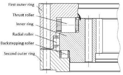
Figure 1.
Structure diagram of main bearing
2.1. Nonlinear Degenerate Model
The traditional safety fatigue criterion requires that the cyclic stress of the general parts is much lower than the yield limit of the material. In every cycle, the damage to the material can also be neglected. Therefore, it is considered that the ultimate strength of the components is a fixed value under a certain cyclic stress. However, in actual work, the main bearing often causes fatigue failure due to manufacturing defects or illegal operation. Periodic stress will cause damage that cannot be ignored for the parts, and this fatigue damage will continue to accumulate and then reduce the structural performance.
Figure 2
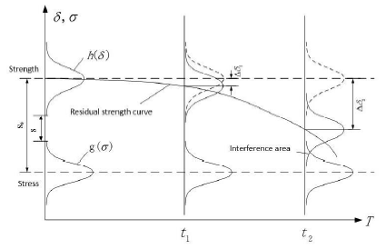
Figure 2.
The dynamic relation between stress and strength
Where $\Delta \delta (t)$ indicates the strength degradation after the working time of the part, $\delta (0)$ indicates the initial strength limit of the material, and $\delta (t)$ represents the residual strength after the time t.
Under the action of dynamic load for a long time, the strength of parts gradually decays. Its residual strength changes with the curve in the diagram, its stress and strength have been interfered at the time ${{t}_{2}}$, and there is an unsafe area. For determining the dynamic reliability of main bearing under cyclic load, it is critical to determine the strength degradation process based on the known load spectrum of spindle load.
In Figure 2, the strength degradation curve is nonlinear, that is, the nonlinear fatigue accumulation theory. The nonlinear fatigue cumulative damage considers that the strength degradation of the material is related to its cyclic stress and its internal damage core. The expression of fatigue damage $D$ is as follows:
Where $m$ is the number of damage cores, $r$ is the damage coefficient, $a$ is the material constant, and $N$ is the equivalent cycle times under the multistage stress, the concrete form of which is:
Where ${{\sigma }_{1}}$ is the maximum stress level in a multi-stage load, ${{N}_{1}}$ is the material’s maximum cycle number under maximum cyclic load, ${{\sigma }_{i}}$ is a certain stress level, ${{\alpha }_{i}}$ is the percentage of cycles under ${{\sigma }_{i}}$ stress, and $d$ is the material constant (needs to be determined experimentally).
From the fatigue mechanism, the defects generated in the early stage of fatigue loading, such as dislocations, slips, voids, etc., have little effect on the strength of the material, but the cracks and propagation processes that are initiated in the later period of the material cause the effective bearing area to decrease. As a result, the strength of the material is rapidly reduced and damage occurs [10].According to the characteristics of fatigue damage, the boundary conditions that the residual strength should be satisfied during the process of material strength degradation are as follows:
(1) The residual strength ${{\delta }_{R}}(0)$ of the material after 0 cycles is equal to the true static tensile strength ${{\delta }_{R}}(0)$ in the material without damage.
(2) After circulating $N$ times under ${{\sigma }_{\max }}$, the residual strength ${{\delta }_{R}}(N)$ is equal to the peak fatigue load ${{\sigma }_{\max }}$, and the material reaches the failure limit.
(3) ${{\delta }_{R}}(n)$ is a monotone increasing function. The fatigue damage of the material needs to meet the thermodynamic irreversible and physical conditions.
According to the fatigue damage boundary condition, considering the effect of stress level $S$ on strength degradation, an exponential degradation model based on experimental strength degradation is introduced [11].
In the equation, $p$ and $q$ are material constants, which can be obtained by the $S-N$ curve of the material.
In the actual working condition, the cyclic stress of the main bearing is mostly random load, and its probability density function is $f(S)$. After the random stress action $n$ times, the residual strength was reducedto ${{\delta }_{R}}(n)$. In the $n$ cycle, the probability of the occurrence of random stress between $[S,S+\text{d}S]$ is $f(S)\text{d}S$, and then the actual number of actions within $[S,S+\operatorname{d}S]$ is:
For the entire area of the distribution of the cyclic stress $S$, by substituting Equation (5) into Equation (4) and integrating it, the strength degradation model of the main bearing under random load is obtained.
In the equation, $\Omega $ is the whole range of the variation of the random stress.
To integrate Equation (6):
In the above equation, the residual strength is a non-linear function of the cyclic stress level, and the parameters $p$ and $q$ need to be obtained by a nonlinear iterative method. However, this test-based method is inconvenient, so consider a simpler way to determine the degradation parameters of the material.
When $n=N$, we get ${{\delta }_{R}}(n)\text{=}S$, and then the equation is expressed as:
The following can be obtained from Equation(8):
Since the cyclic stress level $S$ is small relative to the true tensile strength ${{\sigma }_{b}}$ of the material, ${{S}^{1+q}}$ and ${{\sigma }_{b}}^{1+q}$ will differ by several orders of magnitude, and then ${{S}^{1+q}}$ in Equation (9) can be ignored:
The most common form of the power function describing the material $S-N$ curve [12] is:
From Equations (10) and (11), we can get:
If the material $S-N$ curve is known, the parameters $m$ and $C$ can be obtained by the fitting function, and the material parameters $p$ and $q$ in the strength degradation model can be solved using Equation (12).
For the actual driving of the main bearing, due to the large gap in the texture conditions of different sections and its general work in a number of complex conditions, the main bearing internal load spectrum will also show multi-level fluctuations. Therefore, in actual practice, the main bearing is excavated under multi-level fatigue loads. The main bearing continuously proceeds from one fatigue stress to the next due to the advancement of the rock boring machine until the completion of the excavation or failure occurs.
If the material is subjected to multi-stage cyclic stress ${{S}_{1}},{{S}_{2}},\cdots ,{{S}_{m}}$ before failure, the number of action is ${{n}_{1}},{{n}_{2}},\cdots ,{{n}_{m}}$. After such a process, the residual strength of material can be expressed as:
For determining the cyclic process of the relationship between cyclic stress level $S$ and time $t$, Equation (13) can also be expressed as the relationship between reliability and time, and its specific expression is:
Due to the dispersivity of the material properties and the randomness of the working load, the strength degradation process of the main bearing varies with time and is a random process. Therefore, a stochastic process is introduced to simulate the randomness of the strength degradation under cyclic loading. It is assumed that the stochastic process is a stochastic process with mean ${{\mu }_{x}}$ and standard deviation ${{\sigma }_{x}}$, which are subordinate to the lognormal distribution. Introduce the stochastic process into the intensity degradation model, and then Equation (15) is:
In the $[0,t]$ range, the two sides of Equation (15)are integrated:
Assuming $W(t)=\int_{0}^{t}{X(t)\text{d}t}$, its specific meaning is a stochastic process that describes the integral of the lognormal stochastic process. The specific analytical expression of the distribution function is difficult to obtain. The first order second moment method [13-14] is used to describe the uncertainty of the stochastic process by taking the mean and the variance of both sides of the equation.
Through the approximation of the first order second moment method, the mean and variance of the residual strength after degeneration are obtained. Then, the probability density function of the residual intensity is:
2.2. Structure Fatigue Reliability Model
The load stress of the main bearing is greatly affected by the geological conditions. The sudden change of the stratum within the composite stratum will cause the main bearing contact stress to fluctuate. At the same time, the internal performance of the material is different, and the processing technology will directly affect the performance of the structure. The stress state and ultimate strength of the main bearing will have some dispersion. In general, considering the complexity of the actual working conditions of TBM main bearing and the dispersion of material properties, stress and intensity are random variables distributed in a certain range according to statistical law. If the upper limit of stress is not less than the lower limit of strength, the possibility of failure exists in the structure. Therefore, the stress strength interference model should be introduced to consider the reliability analysis. Figure 3 is a typical stress intensity interference relationship.
Figure 3
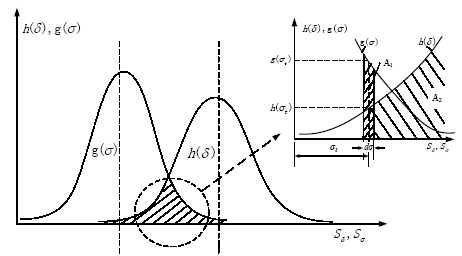
Figure 3.
The stress-strength interference model
It can be seen from the interferogram that the traditional safety factor design, even if the safety factor is greater than 1, still has a certain unreliability. Because the material properties of parts are good and the working stress is stable, the dispersion degree of strength and stress is small, which helps to improve the reliability. Otherwise, it will increase the interference area, resulting in an increase in unreliability. According to the stress strength interference model, it is known that the reliability of a part depends mainly on the degree of stress strength interference. If the distribution model of stress and strength is a known probability distribution, the reliability is expressed as the total probability that the stress is less than the strength, and then the expression is as follows:
In the equation, $\delta $ is the strength limit of the part material and $\sigma $ is the maximum stress of the part.
We can see from the figure that the stress at any time is ${{\sigma }_{t}}$. The continuous distribution of stress was divided in the domain of $-\infty ,+\infty $, such as the area in the diagram $\text{d}\sigma $, and the middle of each small area value represents the regional stress level. The probability of the stress ${{\sigma }_{t}}$ in the area $\text{d}\sigma $ range is as follows (representation of a random event ${{A}_{1}}$):
When the stress is ${{\sigma }_{t}}$, the probability that the strength is greater than the stress is (representation of a random event ${{A}_{2}}$):
The reliability of the calculation of the probability density distribution of the structure’s stress intensity is expressed as:
2.3. System Fatigue Reliability Model
The structure of TBM main bearing is a complex three rows and three column slewing support form, and the failure of the system depends on the failure probability of the roller raceway in each column. The reliability of the bearing system is determined by the working reliability of the three columns internal bearings. The main bearing is defined as safe and reliable only when three columns bearings are in normal state at the same time, so it can be regarded as a series of Bayesian network reliability models [15].For every column bearing, there is a contact between the roller and the inner and outer raceway at the same time, so if one of them has contact fatigue failure, the bearing will also fail. Therefore, it can also be regarded as a simple series reliability model.
It is assumed that the r element reliability matrix is ${{R}_{C}}$, the correlation matrix of the element failure correlation is $A$, the connection matrix is $\Omega $, and the reliability matrix of the main bearing system is $\Gamma $. Therefore, the reliability matrix of the main bearing system can be defined as:
In the equation, $I$ is a unit matrix and ${{R}_{C}}$ includes the main thrust bearing, the backstepping bearing, and the radial bearing. For a series system, the reliability matrix of a component is defined as:
Where ${{R}_{1}},\text{ }{{R}_{2}},\text{ }{{R}_{3}}$ represents the reliability of the main thrust bearing, the back stepping bearing, and the radial bearing respectively.
For ${{R}_{1}},\text{ }{{R}_{2}},\text{ }{{R}_{3}}$ in the upper form, it can also represent the reliability matrix of the three subsystems, which are specifically expressed as:
Where ${{R}_{iI}}\text{, }{{R}_{iO}}$ show the reliability of the contact between the inner and outer raceways of the inner roller in the subsystem $i.$
As with the component reliability matrix, each row in the association matrix represents a component. The element on the main diagonal is 0. The elements not on the main diagonal line are represented by 0 and 1, which represent the failure relationship between two components, respectively. The failure correlation is set to 1, and the failure unrelated is set to 0. If ${{\lambda }_{ij}}$ is used to represent the correlation coefficient between the bearing $i$ and $j$, the association matrix can be transformed into a connection matrix, and the specific form is:
If the system components are completely independent of each other, then ${{\lambda }_{ij}}\text{=}0$, and the connection matrix of the system is a trivial matrix. On the basis of the determination of the reliability matrix and the correlation matrix, the reliability of the main bearing system can be defined as:
3. Engineering Analysis
Taking the main bearing of the rock boring machine in the Dahuofang Reservoir Diversion Project of Liaoning Province as an example, according to the existing cyclic stress level and strength degradation model, the nonlinear degradation simulation of strength is carried out. Then, the reliability of the structure under a given cyclic load is calculated.For the main bearing, the load of the radial roller is smaller and basically remains unchanged, so it does not consider the degradation of its strength and the reliability is set to 1. Therefore, the reliability analysis is mainly aimed at the main roller and backstepping roller under the random composite load.The contact reliability of the two-row roller and the inner and outer raceway is obtained through the above method, and then the correlation matrix between main system and subsystem is established based on the failure correlation. Finally, the overall reliability of the main bearing is obtained.
According to the design requirements, the reliability of the main bearing should be more than 0.9 within 20000 hours of the design life. Because the stratum form is complex during tunneling, according to the literature’s multi load spectrum synthesis method, we can get the probability density function of two main rollers of main bearing under three stage loads.
The maximum contact stress probability density function of the main push roller can be expressed as:
In the same way, the maximum contact stress probability density function of the backstepping roller is as follows:
3.1. Residual Strength Calculation
The materials of the roller and raceway of the main bearing are GCr15 and 42CrMo respectively, which meet the conditions ${{E}_{1}}=209\text{MPa}$, ${{\mu }_{1}}=0.28$, ${{\mu }_{1}}=0.28$, and ${{\mu }_{2}}=0.30$. For the material GCr15 of the main bearing roller, the static tensile strength is 1900MPa. According to the description of the $S-N$ curve in the mechanical engineering material performance data handbook, the survival rate is 99%, and the expression can be expressed as follows:
According to the upperequation, the fatigue parameters $m=11.3266$ and $C=1.3954\times {{10}^{58}}$ can be determined, and the degradation parameters $p=11.3266$ and $q=17.1140$ of the two materials can be obtained.
Using the same method, the expression of the strength degradation process of the race way can be determined as follows:
Assuming that TBM is in turn in the above three strata, the degradation process of its strength can be calculated by its cyclic stress level. The residual strength of the material will also be dispersible under the stress of the logarithmic normal distribution. Therefore, the residual strength of the main bearing structure is simulated according to the normal distribution of the initial strength and the logarithmic normal distribution of the cyclic stress. Based on the contact stress fatigue strength model of the previous article, the simulation results of the residual strength of the roller raceway contact position under the three-stage cyclic loading are shown in Figure 4.
Figure 4
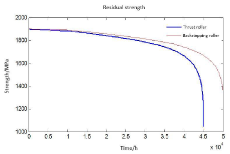
Figure 4.
Residual strength histories of rollers
The remaining strength values of each part of the main bearing are shown in the above 50,000 hours. Because the ultimate tensile strength and cyclic stress are all random variables, the value expressed in the diagram is the residual strength mean value in the degradation process. It is shown that the strength degradation is slow. When the ultimate strength is reduced to about 1,600MPa at the early stage of the main bearing, the strength degradation is speeded up rapidly and the residual strength decreases rapidly, which is consistent with the residual strength experiment in document 8. In fact, the degradation process of the main bearing in each section is also random. The distribution characteristics of residual strength were simulated according to the determined distribution parameters. According to the action time and load cycle characteristics of each section, the random samples of intensity and stress were selected for degradation test, and the sampling frequency was 1/600. The probability density curve of the strength degradation process of the main bearing roller is shown in Figure 5, based on the strength degradation model under the complex working condition of the previous article.
Figure 5
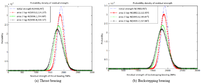
Figure 5.
The probability density curve of residual strength of rollers
3.2. Reliability Method Calculation of TBM Bearing
MATLAB is used to solve the structural reliability of the logarithmic normal distribution of stress and strength. According to the assumption of elasticity in Hertz contact, the contact stress between the roller and the inner and outer raceway is regarded as the same size when the normal pressure acts on the size of the inner and outer raceway. The effect of internal and external contact on reliability is considered through the failure correlation of two pairs of contacts, and the dynamic time process of each reliability is shown in Figure 6.
Figure 6
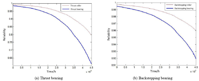
Figure 6.
The reliability of thrust bearings and backstepping bearing
Figure 6 shows the reliability of the trend of the two column thrust bearing main bearing internal and the strength degradation trend of approximation. The subsystem reliability decreases faster than the roller reliability, and with an increase intime the gap is more obvious. According to the design life time of the main bearing, the reliability of the main thrust bearing and the thrust bearing is ${{R}_{1}}=0.9373$ and ${{R}_{2}}=0.9823$ respectively, so the reliability matrix of the main bearing and the thrust bearing is:
In the system, the correlation matrix describing the failure correlation of each component is as follows:
Therefore, the overall reliability of the system is:
In the same way, the dynamic process of time is analyzed for the reliability of the system, as shown in Figure 7.
Figure 7
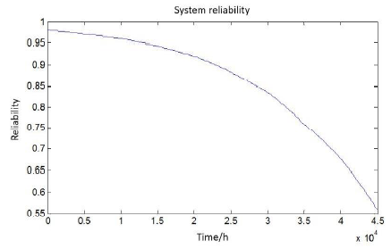
Figure 7.
Residual strength histories of rollers
Figure 7 shows more concretely that the reliability of the main bearing system degenerates slowly at the early stage of work, and the reliability of the system decreases sharply at the later stage of work. This is because in the early stage of service, its strength limit is large and its performance is relatively stable (the dispersion of random strength is small). With the degradation of strength, the residual ultimate strength decreases exponentially and the dispersion of strength gradually increases.In general, to meet the design requirements, the main bearing in the design life is 20000 hours and the reliability is 0.9275, which is greater than 0.9.
4. Conclusions
In this paper, according to the characteristics of contact fatigue failure of the main bearing, a functional function describing the fatigue state of the main bearing is established, and a typical stress-strength interference model is used to analyze the reliability of stress and strength as random variables. Then, according to the complex load conditions of the main bearing and combined with fatigue cumulative damage and residual strength theory, the strength degradation process of the main bearing under varying stress is analyzed, and the dynamic degradation model under complex conditions is established for complex conditions. Based on this, the analytical model of the contact fatigue reliability of the main bearing is obtained. Finally, a failure correlation matrix of main bearing system and internal components is established by combining a fault model tree and Boolean function, and the reliability model of main bearing system considering failure correlation is obtained.
Acknowledgements
This work is sponsored by the Liaoning Province Natural Science Foundation “Study on intelligent processing methods and equipment of rapid and low loss descaling”.
Reference
A Statistical Representation of Fatigue Failure in Solids
,”
Sequential Cumulative Fatigue Reliability,”
A Rational Analytic Theory of Fatigue
,”
First-Order and Second-Order Hybrid Methods for Fatigue Reliability Analysis of Structural Systems
,”A hybrid first--order/second--order method is proposed for fatigue reliability analysis of complicated structural systems. The second order asymptotic formulation for reliability analysis of parallel systems is employed in calculating the fatigue failure probability of the failure path of the system. An equivalent failure element is derived for a failure path by using the concept of equivalent linear safety magin of the parallel system. Fatigue failure probability of the whole system is calculated by modeling the system as a series system combined of equivalent failure elements. Results show that the proposed hybrid method can effectively improve the accuracy of the calculation.
Establishment of Stress Intensity Global Interference Model based on Monte Carlo Method
,”
Intensity Degradation of Metallic Materials under Fatigue Loading
,”
DOI:10.3788/gzxb20103908.1438
URL
[Cited within: 1]

The residual strength is one of the important properties of materials,and it is the basis for predicting fatigue life.It is known that the residual strength is a monotonically decreasing function of the number of loading cycles,and the degradation of the strength is caused by the damage development.The degradation rule of 35CrMo steel is studied based on the development of the damage in the material under cyclic loading and a model to describe the degradation of tensile residual strength of 35CrMo steel is presented.Large amounts of experimental data have been employed to support this model and the comparison between prediction and experiment demonstrates that this model has better capacity of predicting the degradation of tensile residual strength.Three-parameter Weibull function is considered applicable to the distributions of the residual strength after different cycle numbers.However,the parameters of the Weibull distribution are different after different cycle numbers,that is,the parameters of the Weibull distribution changes with cycle numbers.With the cycle numbers increasing,the distribution of residual strength is changing.
Study on Nonlinear Fatigue Damage Cumulative Model based on Binary Fatigue Failure Criterion and its Strength Degradation
,”
Acquisition and Application of S-N Curve for Fatigue Performance of Typical Components
,”
A New Model of Random Fatigue Crack Propagation
,”
Overview of Commonly Used Fatigue Reliability Analysis Methods
,”
Reliability Analysis of Hierarchical System based on Bayesian Network
,”
DOI:10.13224/j.cnki.jasp.2016.06.014
URL
[Cited within: 1]
Reliability modeling of hierarchical systems is significantly difficult because of the complex system structures and imbalanced reliability information at different system levels.A Bayesian network reliability analysis methodology was proposed to model the reliability of binary-state hierarchical systems considering the combination of Bayesian network and Bayesian information aggregation approach to represent the failure relationship among system elements.An example illustrated that,the proposed methodology can significantly improve the accuracy of system-level reliability modeling and reduce the variances of the posterior failure distribution of system by considering the cascading failure dependency and utilizing all available reliability information throughout the system.
