


1. Introduction
For sulfur-containing oil products, the safety problems in production and processing are very serious. The FeS component contained in sulfur-containing oil products often reacts with air during storage and transportation, causing chemical reactions that lead to the release of a large amount of heat and cause many fire and explosion accidents [1-2].
To avoid the occurrence ofsuch malignant events, much research has been conducted in two aspects. On the one hand, many scholars have tried to analyze the reaction mechanism of spontaneous accidents and general reasons of producing Tmax through chemical reaction theories. They proposed that the anti-corrosion coating on the inner wall of the storage tank would be partially peeled off and the iron in the coating would be exposed after the long service cycle. When the sulfur in the crude oil was exposed to a low temperature water-containing environment, the sulfurized rust was generated and the production facilities and tank walls was corroded through chemical and electrochemical modes [3-5]. Furthermore, the sulfurized rust underwent the oxidation reaction with air and released a large amount of heat to incur spontaneous combustion accidents [6-8]. Dou et al. [9-10] studied the chemical reaction mechanism of the self-heating process by analyzing the thermal decomposition kinetics of the sulfurized rust and obtained the thermal decomposition kinetic characteristic parameters and spontaneous combustion mechanism in different stages of the oxidation reaction of the sulfurized rust. With the same conditions in edible oil refining, Landucci [11-13] research ededible oil refining hazards using a thermodynamic model for the estimation of vapor phase composition in storage tanks as a function of operating condition, and this model provides a quick tool for preliminary assessment of hazards due to the formation of flammable mixtures in edible oil storage plants. In addition, the simulation experiments of the self-heating process of sulfurized rust under some special condition shave been conducted to explore the impacts of different factors. At the same time, many researchers adopted experiments to explore the implicit relationship between Tmax and influence factors in the self-heating process. It was obtained from experiments that some factors, including the mass of sulfurized rust, operating temperature, water content of sulfurized rust, air flow rate through the safety valve, oxygen concentration in the safety valve, and pH, had an extremely important impact on the oxidation reaction of sulfurized rust [14-15]. Additionally, the researchers found that 70 ${}^{\text{o}}\text{C}$ is not only the critical temperature at which the chemical reaction takes place but also the temperature of the smoke point, at which SO2is formed. Therefore, 70 ${}^{\text{o}}\text{C}$ is deemed as the threshold temperature for the self-heating process, and when the temperature exceeds 70${}^{\text{o}}\text{C}$, the fire or explosion accidents are triggered [16-18]. However, it is difficult to obtain ${{T}_{\max }}$ of the oxidation self-heating process through experiments because of the lack of accurate or theoretical relation ships between ${{T}_{\max }}$ and multiple uncertainties, namely influence factors. Thus, it is not realistic to quantify the detection and early warning for fire and explosion accidents [19-20].
On the other hand, the modeling method of machine learning was gradually applied to predict ${{T}_{\max }}$ of the oxidation self-heating process based on the relationship between ${{T}_{\max }}$ and the five main factors mentioned above. The Support Vector Machine (SVM) method was first used to build the ${{T}_{\max }}$ prediction model describing the relationship between the rising temperature and various uncertainties in the oxidation process of sulfurized rust based on the experimental dataset in literature [10]. ${{T}_{\max }}$ was obtained from the model based on the SVM method. Compared with the experimental results, the predictive ${{T}_{\max }}$ are within the error ranges. This shows that it is advantageous to study the relationship between ${{T}_{\max }}$ and its influence factors using the machine learning algorithm. In this paper, the Gaussian process regression(GPR) method is adopted to build the ${{T}_{\max }}$ prediction model. Compared with the SVM method, the GPR method has better adaptability to complex nonlinear problems with uncertainties and can make a probabilistic interpretation on the prediction result. Furthermore,the GPR method can meet the accuracy requirements needed in engineering applications and has achieved many successful cases. For example, Samulesson et al. used the GPR method to successfully address the monitoring and fault detection of waste water treatment processes [21]. The GPR method was also successfully applied in short-term wind speed forecasting, solar power forecasting, state-of-charge estimation for batteries, and fault detection [22-25], demonstrating its ability and application prospects to solve practical engineering problems.
In this paper, the GPR method is adopted to model the relationship between ${{T}_{\max }}$ and its influence factors during the oxidation self-heating process of sulfurized rust, and ${{T}_{\max }}$ is predicted using the built model. It is more helpful to solve the nonlinear ${{T}_{\max }}$ prediction problem in the oxidation self-heating process of sulfurized rust, and this will also provide stronger protection for oil and gas production and transport safety.
The remainder of this paper is organized as follows. Section 2 presents our methodology, including data preprocessing, the GPR method, and the model evaluation standard. Section 3 shares a case study on the oxidation self-heating process of the sulfurized rust based on the dataset [10]. Finally, Section 4 provides the conclusion.
2. Methodology
To explore how ${{T}_{\max }}$ occurs in a self-heating process of sulfurized rust, regression methods are adopted. For this purpose, a set of experiments have been conducted at Nanjing Tech University. In the experiments, the five main influence factors mentioned above and ${{T}_{\max }}$ were monitored, and a dataset called set 1, which in cluded 85 samples, was obtained. Our goal is to find the implicit relation ship, as shown in Equation (1) [10], between ${{T}_{\max }}$ and the five factors: water content, mass of sulfurized rust, operating temperature in oil tank, air flow rate, and oxygen concentration in the safety valve.
Where ${{F}_{\text{wat}}}$ [unit:% as mass fraction]=water content of sulfurized rust, ${{M}_{\text{sr}}}$ [unit: g]=mass of sulfurized rust, ${{T}_{\text{ope}}}$ [unit: ${}^{\text{o}}\text{C}$]=operating temperature in oil tank, ${{R}_{\text{air}}}$ [unit: ml/min]=air flow rate through the safety value, and ${{C}_{\text{oxy}}}$[unit: % as volume fraction]=oxygen concentration in the safety value.
In Equation (1), the five factors can be considered as in dependent variables, and ${{T}_{\max }}$ is the dependent variable. The five factors are also considered as the five features to the GPR model, and the data in set 1 must be preprocessed before the GPR model is built.
2.1 Data Preprocessing
During the training process of the GPR model to predict ${{T}_{\max }}$, in order to eliminate the in fluence of the different value ranges among five features on the prediction results, the Z-score normalization method is adopted to standardize the data involved in this paper. The standardized data will improve the training efficiency and prediction accuracy of the GPR model. For example, the feature ${{F}_{\text{wat}}}$ will be standardized through Equation (2) [26]:
Definition: ${{\mu }_{\text{wat}}}$ and ${{\delta }_{\text{wat}}}$ are the mean and standard deviation of feature ${{F}_{\text{wat}}}$ respectively. ${{F}_{\text{wat,}i}}$ is the ith value of the feature ${{F}_{\text{wat}}}$ in the dataset involved in this paper. The other four features ${{M}_{\text{sr}}},\text{ }{{T}_{\text{ope}}},\text{ }{{R}_{\text{air}}},\text{ }{{C}_{\text{oxy}}}$, and ${{T}_{\max }}$ will conduct the same data pre-processing as ${{F}_{\text{wat}}}.$
The 85 samples in set1 are divided into the training set and the testing set, which are used to train and test the GPR model respectively. For obtaining a good GPR model, it is needed that all the minimum and maximum values of the five features and ${{T}_{\max }}$ in the dataset should be included in the training set. In addition, in order to prevent the GPR model from overfitting, the number of the samples included in the training set is supposed to be less than 80% of the total set [27-28]. Therefore, 60 samples in set1 (nearly 70%) are chosen to train the GPR model, and the remaining 25 samples are used to test the GPR model for the prediction of ${{T}_{\max }}$ in this paper. The additional 17 samples in literature [10], called set2,are used to further verify the generalization and effectiveness of the GPR model. We can see the change of ${{T}_{\max }}$ in different conditions from Figure 1.
Figure 1
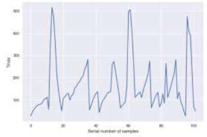
Figure 1.
The ${{T}_{\max }}$ corresponding to each sample
2.2. The Theory of Gaussian Process Regression
Fora regression problem, it is usually assumed that there is a training set D with n observations expressed as
$D=\left\{ \left( {{\mathbf{x}}_{1}},{{y}_{1}} \right),\left( {{\mathbf{x}}_{2}},{{y}_{2}} \right),\cdots ,\left( {{\mathbf{x}}_{n}},{{y}_{n}} \right) \right\}$
Let ${{\mathbf{x}}_{i}}=\left[ {{x}_{i1}},{{x}_{i2}},\cdots ,{{x}_{id}} \right]$ and $i=1,2,\cdots ,n$, $\mathbf{X}={{\left[ {{\mathbf{x}}_{1}},{{\mathbf{x}}_{2}},\cdots ,{{\mathbf{x}}_{n}} \right]}^{T}}$, $\mathbf{y}={{\left[ {{y}_{1}},{{y}_{2}},\cdots ,{{y}_{n}} \right]}^{T}}.$ The task of the regression is to learn the mapping relationship $\left( f\left( \bullet \right)|\mathbf{X}\mapsto \mathbf{y} \right)$ between $\mathbf{X}$ and $\mathbf{y}$ based onthe training set D and to predict the most likely output value ${{f}_{*}}$ corresponding to the input point ${{x}_{*}}$ via the mapping relationship.
The above assume that the training set also holds true for the use of Gaussian processes(GPs) to solve regression problems. Generally, from the perspective of the function space, we define a GP to describe the distribution of function and make a Bayesian inference directly in the function space [29-30]. A GP is a set of limited random variables with joint Gaussian distribution and is determined by its mean function and covariance function completely. An $f\left( \mathbf{x} \right)$’s mean function and covariance function can be defined as
Therefore, a GP can be written as
Where $E \left( \bullet \right)$ denotes the operator of expectation.
In general, observation data ${{y}_{i}}$ can be described by the underlying function $f\left( {{\mathbf{x}}_{i}} \right)$, which is corrupted by noise $\delta $ for real-world regression problems. This can be defined as
Where $f\left( {{\mathbf{x}}_{i}} \right)$ and $\delta$ are two independent GPs, and $\delta$ is a GP with mean 0 and variance $\sigma _{n}^{2}.$
Therefore, the prior distribution of $\mathbf{y}$ can be expressed as
Meanwhile, the joint prior distribution of observations $\mathbf{y}$ and predictions ${{\mathbf{f}}_{\mathbf{*}}}$ is
Where ${{\mathbf{X}}_{\mathbf{*}}}$ denotes a ${{n}_{*}}\times d$ matrix of prediction set. For the input dataset $\mathbf{X}$ with $n$ samples and the prediction dataset ${{\mathbf{X}}_{\mathbf{*}}}$ with ${{n}_{*}}$ samples, ${{K}_{*}}=K\left( \mathbf{X,}{{\mathbf{X}}_{*}} \right)$ expresses a $n\times {{n}_{*}}$ matrix of covariance between the input and prediction samples. The same calculation rule is endowedwith $K=K\left( \mathbf{X,X} \right)$, ${{K}_{**}}=K\left( {{\mathbf{X}}_{\mathbf{*}}}\mathbf{,}{{\mathbf{X}}_{*}} \right)$,and $K_{*}^{T}=K{{\left( \mathbf{X,}{{\mathbf{X}}_{*}} \right)}^{T}}.$ ${{\mathbf{I}}_{n}}$ is the identity matrix. ${{\mathbf{f}}_{\mathbf{*}}}$ denotes the most likely output values corresponding the prediction dataset ${{\mathbf{X}}_{\mathbf{*}}}$.
Because the joint prior distribution of observations $\mathbf{y}$ and predictions ${{\mathbf{f}}_{\mathbf{*}}}$ is normal distribution, the posterior distribution of predictions ${{\mathbf{f}}_{\mathbf{*}}}$ can be directly calculated as
Where
${{\overline{\mathbf{f}}}_{\mathbf{*}}}$ and $\operatorname{cov}\left( {{\mathbf{f}}_{*}} \right)$ are respectively the mean and covariance of predictions ${{\mathbf{f}}_{\mathbf{*}}}$ corresponding to the prediction dataset ${{\mathbf{X}}_{\mathbf{*}}}$. Therefore, the posterior distribution of predictions ${{\mathbf{f}}_{\mathbf{*}}}$ will be obtained.
Various covariance functions can be selected when the GPR model is used to solve such problems. The most common covariance function is the squared exponential kernel:
Where $\theta =\left\{ l,\sigma _{_{f}}^{2},\sigma _{_{n}}^{2} \right\}$ is the parameter set of the GPR modeland is also called its hyper-parameters. $l$ is the length-scale, $\sigma _{_{f}}^{2}$ is the signal variance, and $\sigma _{n}^{2}$ is the noise variance. As we know, the simplest way to obtain the GPR model’s hyper-parameters $\theta $ is to maximize the log-likelihood function of the data set as shown in Equation (12):
The optimal hyper-parameters will be gotten through the above calculation. Then, Equations (9) and (10) will be used to calculate ${{\overline{\mathbf{f}}}_{\mathbf{*}}}$ and $\operatorname{cov}\left( {{\mathbf{f}}_{\mathbf{*}}} \right)$.
The following is the pseudo-code of the GPR algorithm according to the theory above:
Where a single prediction point ${{\mathbf{x}}_{\mathbf{*}}}$ is used in this pseudo-code, $\mathbf{\alpha }={{\left( K+\mathbf{\sigma }_{n}^{2}{{\mathbf{I}}_{n}} \right)}^{-1}}\mathbf{y}$, and $cholesky\left( K+\mathbf{\sigma }_{n}^{2}{{\mathbf{I}}_{n}} \right)$ denotes Cholesky decomposition.
2.3. Evaluation Criterion of GPR Model
To assess the prediction performance of the GPR model, we introduce a score function to quantitatively evaluate the performance of the GPR model that is relative to the training set, test set, and validation set. The score values indicate the robustness and accuracy of the GPR model. The closer the score value of the score function is to 1, the better the GPR model. The score values may be negative if the GPR model is bad enough. The specific expression of the score is
Where $u=\sum\limits_{l=1}^{N}{{{\left( {{T}_{\max ,\exp ,l}}-{{T}_{\max ,gpr,l}} \right)}^{2}}}$ and $v=\sum\limits_{l=1}^{N}{{{\left( {{T}_{\max ,\exp ,l}}-{{\overline{T}}_{\max ,\exp }} \right)}^{2}}}.$ ${{T}_{\max ,\exp ,l}}$ and ${{T}_{\max ,gpr}}_{,l}$ denote the lth experimental value and the predictive value of ${{T}_{\max }}$ respectively. ${{\overline{T}}_{\max ,\exp }}$ denotes the mean of all ${{T}_{\max ,\exp ,l}}.$ $N$ denotes the number of samples in the training set, the test set, and the validation set respectively.
Meanwhile, the variable $\sigma $, defined as the mean relative error between ${{T}_{\max ,\exp }}$ and ${{T}_{\max ,gpr}}$ and shown in Equation (14), is also used to measure the performance of the GPR model, and the GPR model will demonstrate better performance if $\sigma $ has a lower value.
Where M denotes the number of all samples included in the training set, the test set, and the validation set.
3. Application and Result Discussions
3.1. Training and Testing of the GPR Model
When the GPR model is used to predict ${{T}_{\max }}$, the five features in the training set are inputted to the GPR model, and ${{T}_{\max }}$ is the model out put. According to the deviation between the model output and the maximum temperature measured by experiments, the GPR model is trained. In order to evaluate the performance of the trained GPR models, the data in the test set is inputted to the trained GPR models, and the obtained values of score and $\sigma$ will determine the best-suited GPR model. Further, the 17 samples in set2, called the validation set, are similarly used to validate the best GPR model through the values of score and $\sigma$. All the above work, including model training, data preprocessing, and model evaluation, are based on the programming language of python and relative machine learning package such as scikit-learn, pandas, and Numpy [26, 31].
3.2. Results and Discussions
For the training set and the test set in set1, the experimental ${{T}_{\max }}$ versus the predicted ${{T}_{\max }}$ by the GPR model are shown in Figure 2(a) and Figure 2(b)respectively. The experimental ${{T}_{\max }}$ versus the predicted ${{T}_{\max }}$ by the GPR model for set 2 is presented in Figure 2(c). The evaluation parameter values of $score $, $R$, and $\sigma$ of the GPR model are shown in Table 1.R denotes the correlation coefficient.
Figure 2
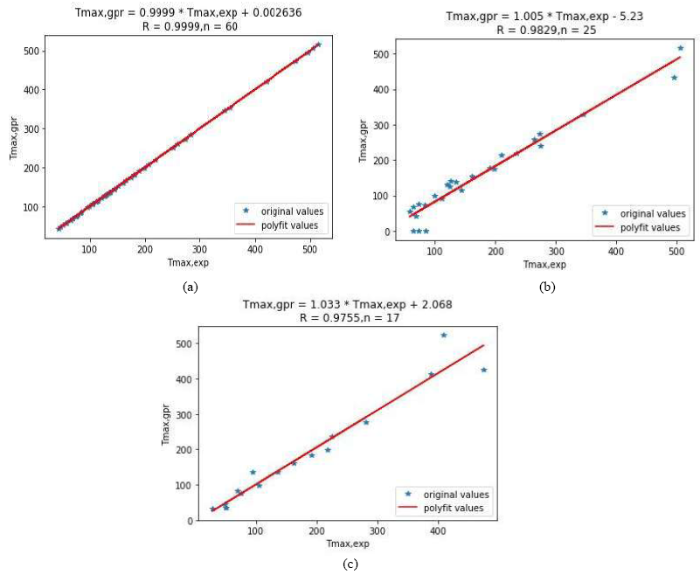
Figure 2.
(a) Correlation between the ${{T}_{\max ,\exp }}$ and ${{T}_{\max ,gpr}}$ for the training set;(b) Correlation between the ${{T}_{\max ,\exp }}$ and ${{T}_{\max ,gpr}}$ for the test set;(c) Correlation between the ${{T}_{\max ,\exp }}$ and ${{T}_{\max ,gpr}}$ for the validation set
Table 1 GPR model evaluation parameter values
| Dataset | $score $ | $R$ | $\sigma $ | |
|---|---|---|---|---|
| set1 | Training set | 0.9999 | 0.9999 | 5.4972 |
| Test set | 0.9606 | 0.9829 | ||
| set2 | Validation set | 0.9497 | 0.9755 | |
From the results shown in Figure 2(a), Figure 2(b), and Table 1, we can see that the GPR model shows excellent prediction performance on the training set and test set, especially on the training set, and the values of the score and R values are all over 0.9. Although the relative error of the test set is larger than the training set due to some poor fitting points, the predictive performance is still good for set1. As for the poor fitting points shown in Figure 2(b), the reason may be due to experimental mistakes or singularities [10]. No one can conquer the curse of original data for any regression model unless we eliminate the anomalous data in order to train a remarkable model.
For the validation set, the performance of the GPR model is not as good as set1. Not only is the score value in set 2significantly less than that in set1, but there are also several points that deviate sharply from the fitting curve, as shown in Figure 2(c). This indicates that the performance of the GPR model declines for set 2. The reasons may be due to factors such as experimental conditions, raw materials, and operation rules inset2.
Given the water content and the mass of sulfurized rust, operating temperature in the oil tank, air flow rate, and oxygen concentration in the safety valve, the prediction performance of ${{T}_{\max }}$ by the GPR model decreases sequentially on the training set, test set, and validation set. The prediction performance especially decreases on the validation set. However, the GPR model has high correlative values over 0.97 between ${{T}_{\max ,\exp }}$ and ${{T}_{\max ,gpr}}$, and the score values are very close to 1 on each dataset. For comparison, we also obtained the related results using the SVM model for the same problem, as shown in Table 2.
Table 2 SVM model evaluation results [10]
| Dataset | score | R | σ | |
|---|---|---|---|---|
| set1 | Training set | 0.998 | 0.996 | 6.2894 |
| Test set | 0.950 | 0.976 | ||
| set2 | validation set | 0.940 | 0.968 | |
Evidentially, from the model evaluation results in Table 1 and Table 2, we can gain that the ${{T}_{\max }}$ prediction performance of the GPR model is superior to that of the SVM model in the score of score function, $R$ and the mean relative error between ${{T}_{\max ,\exp }}$ and ${{T}_{\max ,gpr}}.$ This proves the advantages of the GPR model in dealing with the problems of nonlinear uncertainties. It also verifies that the GPR method is more suitable for modeling observations with noise. Further, due to the more accurate predictions of ${{T}_{\max }}$ by the GPR model, it will be more favorable for sounding an alarm or initiating an automatic protection system for a fire or an explosion in an oil tank.
4. Conclusions
In this paper, the Gaussian process regression (GPR) method was applied to model the prediction of the maximum temperature (${{T}_{\max }}$) during the oxidation self-heating process of sulfurized rust. Five factors that have main effect son ${{T}_{\max }}$, such as water content, mass of sulfurized rust, operating temperature in the oil tank, air flow rate, and oxygen concentration in the safety value, are used as inputs of the GPR model. The validity and rationality of the GPR model are not only verified by the model parameter evaluation value based on the training set, test set, and validation set, but also compared with the SVM modelling results to reflect the excellent performance of the GPR. The GPR model achieves more accurate prediction of ${{T}_{\max }}$ than the SVM model, and it is more favorable for reducing the risk of fire and explosion of crude oil in production and transportation and preventing accidents.
Acknowledgements
The authors of this paper would like to thank Peng Hou and others in the State Key Laboratory of Explosion Science and Technology for providing an experimental space and technical support.
Reference
Thermal Analysis on the Kinetics of Thermal Decomposition of Sulfurized Rust
,”
The Influence of Sulfurization of Rust in Oil Tanks
,”
DOI:10.1080/00908310600623496
URL
[Cited within: 1]

Hydrogen sulfide reacts with the corrosion products (Fe2O3) in oil tanks to form iron sulfides. The oxidation and released heat of iron sulfides can lead to spontaneous combustion of iron sulfides and fire of oil tanks. In this article, the simulating production process of iron sulfides in oil tanks and the effects of flow rate of hydrogen sulfide, environmental temperature and setting time on the quantities and types of iron sulfides are studied.
Kinetic Analysis for Spontaneous Combustion of Sulfurized Rust in Oil Tanks
,”
DOI:10.1016/j.jlp.2014.10.003
URL
[Cited within: 1]
In order to evaluate the spontaneous combustion hazards of sulfurized rust in oil tanks, one kind of rust was obtained from respiratory valve inner cavity of a crude oil tank in a petrochemical company. The rust was sulfurized in sulfuration experimental apparatus. The production was analyzed by X-ray energy dispersive spectrometry (EDS), scanning electron microscopy (SEM) and then thermo-gravimetric analysis (TGA). The EDS result shows that the main substances are FeS and FeS2 which are liable to spontaneous combustion. The sulfurized rust gives a short length of side and diamond appearance, and a large pore size in structure based on X-ray Diffraction (XRD). The whole oxidation process has three complex stages. The corresponding apparent activation energy values, most probable mechanism functions and pre-exponential factor values were calculated by Madhusudanan-Krishnan-Ninan method and the master plot method. The results indicate that the first and third stages of mass loss are up to the power function mechanism, but the second stage accords with the nucleation and nucleus growth mechanism. The values of apparent activation energy increase successively from the first stage to the third stage. The second stage has the maximum pre-exponential factor value, while the first has the minimum. With the obtained parameters above, the oxidation process of sulfurised rust could be simulated, which would benefit for monitoring and early warning of oil tanks. (C) 2014 Elsevier Ltd. All rights reserved.
Oxidation Experiment of Sulfurized Rusts in Crude Oil Tank
,”The oxidation process of sulfurized rusts was investigated.Some iron oxides collected from inner cavity of respiratory valve equipped on the roof of a crude oil tank were put into the self-made sulfurization and oxidation experimental apparatus to gain wet and dry sulfurized rusts.Their chemical compositions and phase were analyzed by energy dispersive spectrometer( EDS) and scanning electron microscope( SEM).Results showed that both of wet and dry sulfurized rusts had S,Fe_2O_3,Fe_3S_4 and FeS_2,with FeS only existed in wet sulfurized rusts.The two kinds of rusts gave a short length of side,diamond appearance and a large pore size in structure.The oxidation process of wet sulfurized rusts was investigated including electrochemical reaction stage,electrochemical chemical reaction coexisting stage,and chemical reaction stage.The oxidation product of wet sulfurized rusts was Fe_2O_3.On the basis of the results,an indicator for monitoring and early-warning was proposed to prevent the accidental vessel or tank from fire and explosion.
Study on Spontaneous Combustion Mechanism of Oil Containing Sulfur based on Thermal Analysis
,”By making use of Q600 Simultaneous TO-DSC.thermal analysis experiments of 5 FeS samples with different diameters are completed.Spontaneous combustion mechanism of the oil containing sulfur is researched based on the experimental results of TG and DSC.Experimental results show that FeS sample is not sensitive to the change of temperature.In generally,oxidative temperature of FeS sample is more than 250 and oxidative rate is slow,Sample diameter plays an important role in oxidative tendency of FeS sample.With the increase of sample diameter,the oxidative temperature of FeS sample increases and the range of oxidative temperature expands.Heating rale also influences on oxidalive tendency of FeS sample and the oxidalive tendency is more obvious in case of slow healing rate.
Synthesis of Pyrophoric Active Ferrous Sulfide with Oxidation Behavior under Hypoxic Conditions
,”
DOI:10.1016/j.vacuum.2017.07.001
URL
[Cited within: 1]
Ferrous sulfide produced by rust sulfuration in crude oil tank can cause accidents such as fire and explosion when exposed to air. It is quite difficult to determine the specific location of the sulfur corrosion products in crude oil tanks as well as to acquire for laboratory testing. Thus, ferrous sulfide with high spontaneous combustion activity is a good alternative for continuing the research of sulfur corrosion products. In this study, pyrophoric active ferrous sulfide sample was synthesized in laboratory. The synthetic sample was studied by X-ray diffraction (XRD), scanning electron microscopy (SEM) combined with energy dispersive spectrometer (EDS), electron probe microanalysis (EPMA) and thermal analysis (TA), respectively. The tests indicated that the synthetic sample was amorphous flocculent agglomerate and the atomic ratio of Fe and S was 1:1 approximately, and the oxidative product was mainly Fe 2 O 3 . Non-isothermal calorimetric experiments were conducted with different heating rates. The reaction atmosphere was hypoxic with a 5:95% oxygen:nitrogen gas mix. Apparent activation energy was estimated based on iso-conversional methods. It would benefit for safety on petrochemical industries such as monitoring and early warning of fire and explosion of oil tanks caused by ferrous sulfide with the obtained parameters.
The Generation of Pyrophoric Material in the Cargo Tanks of Crude Oil Carriers
,”
Study on Dynamic Ignition Temperature Curve of Oil Storage Tank Induced by Ferrous Sulfide
,”
DOI:10.1007/BF02911031
URL
[Cited within: 1]
By inference, the ignition of the oil storage tank is caused by the oxidation of ferrous sulfide produced from the sulfur corrosion. The formation process of ferrous sulfide in oil storage tank is described. The spontaneous oxidation process of ferrous sulfide is tracked for 19 hours by spontaneous ignition heat isolation test system to observe the variation characteristics of dynamic temperature changes during the oxidation process of ferrous sulfur under isolated heat. The experiment show that the oxidation process of ferrous sulfide may proceed in three stages, i.e. motivation oxidation, medium speed oxidation and accelerative oxidation stages. In the motivation oxidation stage, the energy is accumulated, and the ferrous sulfide is activated. The temperature of the sample basically is not changed. In the medium speed oxidation stage, the molecules on the surface of ferrous sulfide sample are activated, and the oxygen adsorbed on the surface of ferrous sulfide sample motivates the oxidation process. The sample temperature elevates rather slowly. In the accelerative oxidation stage, the interior ferrous sulfide molecules are activated and proceed the oxidation process. The temperature rises rapidly. The results show that as the reaction proceeds, the variation extent of temperature varies much bigger. The reaction heat of oxidation could not disperse in time, instead, it is accumulated and the temperature rises rapidly causing the spontaneous combustion of the oil. In addition, the X ray diffraction graph and temperature curve prove that water plays an important role in the oxidation of ferrous sulfide.
Analysis on Oxidation Process of Sulfurized Rust in Oil Tank
,”
DOI:10.1007/s10973-016-5884-x
URL
[Cited within: 1]
The paper focuses on the oxidation process of sulfurized rust in crude oil tank. Firstly, one sort of rust was put into the sulfurization and oxidation experimental apparatus. The chemical composition
SVM Application in Hazard Assessment: Self-Heating for Sulfurized Rust
,”
DOI:10.1016/j.jlp.2015.11.011
URL
[Cited within: 7]
61The support vector machine (SVM) technique is applied in order to predict the maximum temperature (Tmax) of oxidation self-heating process for the first time.61Five governing parameters are selected, i.e. the water content, mass of sulfurized rust, operating temperature, air flow rate and oxygen concentration in the respiratory/safety valve.61The maximal temperatures (Tmax) values calculated by SVM technique were in good accordance with the experimental results.61The prediction of accidents due to the oxidative self-heating is also presented.
Hazards and Safety Issues Associated to the Residual Solid Content in Crude Edible Oil Processing
,”
Hazard Assessment of Edible Oil Refining: Formation of flammable Mixtures in Storage Tanks
,”
DOI:10.1016/j.jfoodeng.2011.02.011
URL
This work presents a methodology for the assessment of hazards due to the formation of flammable mixtures in edible oil refineries, with particular focus on storage tanks. Safety issues in these plants are due to the presence of residual volatile flammable solvents deriving from the extraction processes, which may accumulate in the storage tanks and generate flammable vapour mixtures. The methodology, based on the application of a thermodynamic model for the estimation of vapour phase composition in oil storage tanks as a function of operating conditions (i.e. temperature and residual solvent content), allows the identification of potential hazards due to formation of flammable mixtures inside the tanks. The model was first validated using available experimental data and then extended to case-studies representative of state-of-the-art industrial storage applications. The results of the case-studies were then used to calculate specific hazard indexes, providing a quick tool for preliminary assessment of hazards due to the formation of flammable mixtures in edible oil storage plants.
Analysis of Maintenance and Storage Operations in Edible Oil Plants: Formation of Flammable Mixtures
,” in
Study of Spontaneous Combustion Mechanism and Heat Stability of Sulfide Minerals Powder based on Thermal Analysis
,”
DOI:10.1016/j.powtec.2016.12.040
URL
[Cited within: 1]
The spontaneous combustion mechanism of sulfide minerals powder is studied by simultaneous thermal analysis. The chemical reactions of pyrites in the atmospheres of air and nitrogen are deduced and the corresponding reaction products are characterized by the Raman spectroscopy. The characteristic temperatures of the pyrite reaction process are discussed in different conditions. The results show that the process of oxidation spontaneous combustion can be divided into three stages. Fe 3 FeSiO 4 (OH) 5 in the minerals is decomposed at low temperature in the oxidation process. FeS 2 , the main component of the mineral, is mainly oxidized in the stage of oxidation spontaneous combustion. However, FeS 2 will be decomposed under heating in nitrogen atmosphere. Thermal stability of pyrite in air is lower than that in nitrogen, and its thermal stability will be improved by increasing heating rate and particle size.
Mechanism of Mechanical Activation for Spontaneous Combustion of Sulfide Minerals
,”
DOI:10.1016/S1003-6326(13)62457-7
URL
[Cited within: 1]
In order to uncover the intrinsic reasons for spontaneous combustion of sulfide minerals, representative samples were collected from typical metal mines to carry out the mechanical activation experiment. The structures and heat behaviors of activated samples were characterized by scanning electron microscopy (SEM), X-ray diffraction (XRD) analysis, and simultaneous thermal analysis (STA). It is found that the sulfide minerals after mechanical activation show many changes with increased specific surface areas, aggregation phenomenon, decreased diffraction peak intensity, broadened diffraction peak, declined initial temperatures of heat release and self-ignition points. A new theory for explaining the spontaneous combustion of sulfide minerals is put forward: the chemical reaction activity of sulfide minerals is heightened by all kinds of mechanical forces during the mining, and the spontaneous combustion takes place finally under proper environment.
Pyrophoric Oxidation of Iron Sulphide
,”
DOI:10.1016/0257-8972(88)90078-3
URL
Mackinawite, which is formed in the cargo tanks of oil tankers by the reaction between rust and hydrogen sulphide, has been shown to oxide by a two-stage process. This paper reports that the time interval between the two stages corresponds with the evaporation of the bulk water which was necessary before pyrophoricity. The oxidation of dried samples of 3 g weight was pyrophoric when the relative humidity of the air was above about 50% but slow and controlled below 50% humidity. The presence of moisture doubled the rate of the controlled oxidation which was a first-order reaction.
Risk Forecast of Spontaneous Combustion of Sulfide Ore Dump in a Stope and Controlling Approaches of the Fire
,”
Study on the Effect of Water on the Formation and Pyrophoricity of Ferrous Sulfide
,”
DOI:10.1080/10916460903585949
URL
[Cited within: 1]
Rust formed by corrosion on the inner surfaces of oil tanks can react with humidity-saturated hydrogen sulfide. The reactions produce pyrophoric ferrous sulfide and can cause fire and explosions when exposed to air during production or maintenance. Water content has an important effect on both the formation and the pyrophoricity of ferrous sulfide and the effect was investigated in detail in this article. The experimental results showed that water is involved in oxidation reaction of ferrous sulfide and enhances the pyrophoricity, making ferrous sulfide more dangerous and able to easily cause fire or explosion accidents.
New Approach to Study Iron Sulfide Precipitation Kinetics, Solubility, and Phase Transformation
,”
DOI:10.1021/acs.iecr.7b01615
URL
[Cited within: 1]
A reliable anoxic plug flow reactor has been developed to study iron sulfide (FeS) precipitation kinetics, solubility, and phase transformation simultaneously. The effects of temperature (23–125 °C), ionic strength (0.00886–5.03 mol/kg), and ferrous iron [Fe02(II)] to sulfide [S02(-II)] concentration ratio (1:20 to 1:5) were studied. The kinetics of FeS precipitation was found to be a pseudo-first-order reaction with respect to Fe02(II) concentration, when Fe02(II) concentration is significantly lower than the S02(-II) concentration. FeS precipitation kinetics can be accelerated by high temperature and high ionic strength but not be affected by the Fe02(II) to S02(-II) concentration ratio at the tested ratio range. A model for predicting FeS solubility and precipitation was developed by using FeS solubility data measured in this study and data from literature. At a temperature ≤100 °C, freshly precipitated FeS was found to be mackinawite. Mackinawite can transform to troilite at a temperature ≥50 °C, and low ionic strength favors the phase transformation. Also, mackinawite formed from steel corrosion seems to be easier to transform to troilite than the mackinawite formed from precipitation. This study presented a new approach for iron sulfide study and contributed valuable FeS thermodynamics and kinetics data for FeS prediction and control in industry.
Gaussian Process Regression for Monitoring and Fault Detection of Wastewater Treatment Processes
,”
DOI:10.2166/wst.2017.162
URL
PMID:28659535
[Cited within: 1]
Monitoring and fault detection methods are increasingly important to achieve a robust and resource efficient operation of wastewater treatment plants (WWTPs). The purpose of this paper was to evaluate a promising machine learning method, Gaussian process regression (GPR), for WWTP monitoring applications. We evaluated GPR at two WWTP monitoring problems: estimate missing data in a flow rate signal (simulated data), and detect a drift in an ammonium sensor (real data). We showed that GPR with the standard estimation method, maximum likelihood estimation (GPR-MLE), suffered from local optima during estimation of kernel parameters, and did not give satisfactory results in a simulated case study. However, GPR with a state-of-the-art estimation method based on sequential Monte Carlo estimation (GPR-SMC) gave good predictions and did not suffer from local optima. Comparisons with simple standard methods revealed that GPR-SMC performed better than linear interpolation in estimating missing data in a noisy flow rate signal. We conclude that GPR-SMC is both a general and powerful method for monitoring full-scale WWTPs. However, this paper also shows that it does not always pay off to use more sophisticated methods. New methods should be critically compared against simpler methods, which might be good enough for some scenarios.
Fault Prognosis of Filamentous Sludge Bulking Using an Enhanced Multi-Output Gaussian Processes Regression
,”
Battery State-of-Charge Estimation based on Regular/Recurrent Gaussian Process Regression
,”
DOI:10.1109/TIE.2017.2764869
URL
State of charge (SoC) estimation is of key importance in the design of battery management systems. An adaptive SoC estimator, which is named AdaptSoC, is developed in this paper. It is able to estimate the SoC in real time when the model parameters are unknown, via joint state (SoC) and parameter estimation. The AdaptSoC algorithm is designed on the basis of three procedures. First, a... [Show full abstract]
Short-Term Solar Power Forecasting based on Weighted Gaussian Process Regression
,”
DOI:10.1109/TIE.2017.2714127
URL
Photovoltaic (PV) power is volatile in nature and raises level of uncertainty in power systems. PV power forecasting is an important measure to solve this problem. It helps to improve the reliability and also reduces the generation cost. Advances in computer technology and sensors make the numeric modeling methods a hotspot in the field of PV power forecasting. However, data modeling methods strongly rely on the accuracy of measurement data. Unavoidable outliers in the measured meteorological data have an adverse effect on the model due to their heteroscedasticity. Although many studies can be found focusing on outlier detection, but only a few have incorporated outlier detection with regression models. In this study, an innovative method employing weighted Gaussian process regression (WGPR) approach is proposed, such that data samples with higher outlier potential have a low weight. A density-based local outlier detection approach is introduced to compensate the deterioration of Euclidean distance for high-dimensional data. A novel concept of the degree of nonlinear correlation is incorporated to compute the contribution of every individual data attribute. Effectiveness of the proposed method is demonstrated by performing experimental analysis and making comparisons with other typical data-based approaches, and the results exhibit higher estimation accuracy.
Short-term Wind Speed Forecasting based on Gaussian Process Regression Model
,”The short-term wind speed forecasting is very important for the operation of grid-connected wind power generation systems.The accuracy forecasting of the wind speed can also effectively reduces or avoids the adverse effect of wind farm on power grid,meanwhile,strengthens competition ability of wind farm in electricity market.In order to improve the forecasting accuracy,a wind speed forecasting method based on the Gaussian process(GP) was proposed.Firstly,the embedding dimension and the delay time of the wind speed time series were respectively calculated by autocorrelation method and false neighbor method,the phase space reconstruction of the chaotic wind speed time series was received.Then,the reconstructed wind speed time series was predicted by the GP model,at the same time the "super parameter" in the covariance function was determined under the Bayesian framework.Finally,wind speed time series was used to predict by the trained GP,which was compared with support vector machine(SVM),least squares support vector machine(LSSVM) and BP neural network(BPNN).The simulation results show that GP predict model can be used to accurately predict and has stable performance.So it can be widely used in engineering practice.
Why Validation Matters: A Demonstration Predicting Antipsychotic Response Using 5 Rcts
,”
Principles of QSAR Models Validation: Internal and External
,”
Machine Learning of Linear Differential Equations Using Gaussian Processes
,”
DOI:10.1016/j.jcp.2017.07.050
URL
[Cited within: 1]
Abstract: This work leverages recent advances in probabilistic machine learning to discover conservation laws expressed by parametric linear equations. Such equations involve, but are not limited to, ordinary and partial differential, integro-differential, and fractional order operators. Here, Gaussian process priors are modified according to the particular form of such operators and are employed to infer parameters of the linear equations from scarce and possibly noisy observations. Such observations may come from experiments or "black-box" computer simulations.
