


1. Introduction
The technical state of an engine will deteriorate with an increase in use time. In the case of armored equipment engines, the traditional method is generally used to measure the technical state by motor hours [1], and periodic maintenance is carried out for the same type of engine based on a fixed number of motor hours. However, due to different factors such as the use environment, the users, and the intensity of use, the recorded motor hours sometimes cannot fully reflect the actual technical states of all the engines of the same model. In this case, the implementation of periodic maintenance can easily lead to “surplus maintenance” or “insufficient maintenance” [2], so it is necessary to consider achieving condition based maintenance (CBM). Life prediction is the basis for the realization of CBM [3], and it is the key technology to make regular preventive maintenance and corrective maintenance into the foreseeable CBM.
The research on life prediction at present mainly focuses on single-parameter prediction of a single machine. The research methods mainly analyze and predict based on probability or mathematical statistics by collecting data, or they predict a certain part based on the expansion of micro cracks [4]. The former needs to use a large number of samples for full life test to collect the full life data, while the latter needs to analyze and determine the complex failure mechanism and process of the product. With the increasing level of science and technology, more and more products with long life and high reliability have appeared in the fields of aviation, aerospace, and military industry. These products are difficult to fail in a short period of time even in accelerated life tests [5]. In this case, the use of a large number of samples for full life test is time-consuming and laborious, and the failure mechanism of the product is complex and difficult to determine. In view of this, it is no longer feasible to use the traditional reliability analysis method for life prediction.
Degradation data refers to the data of equipment performance, state, and other parameters that gradually deteriorate with an increase in use time. In the process of equipment use and testing, it is easy to obtain degradation data through in-vehicle instrumentation, BIT devices, and sensor measurements, and then artificial intelligence algorithms such as neural networks can be adopted to carry out reasoning for life prediction and maintenance decisions.
This method of life prediction based on degradation data and intelligent algorithms does not require full life data, nor does it consider the failure mechanism of the product. Instead, it treats the degradation process as a “black box” [6]. The reliability analysis and state maintenance decision can be carried out by using the backward correlation of the degradation data and the powerful reasoning calculation function of the intelligent algorithm to solve the problem of “surplus maintenance” or “insufficient maintenance” in the traditional maintenance mode of equipment; moreover, it meets the maintenance requirements under the condition of informationization. In this paper, the Principal Component Analysis (PCA) method is used to combine multiple degradation parameter data into one comprehensive parameter data, and then the BP neural network algorithm is used to realize multi-parameter life prediction.
2. Theoretical Analysis
2.1. Principle of Neural Network Trend Prediction
The prediction problems of neural networks are mainly divided into two types: the trend prediction of time series relations and the regression prediction of causality. Neural network trend prediction is a prediction method that reflects the rule and relationship of a prediction variable by collecting and analyzing the historical data of a prediction variable, and then it carries out trend extrapolation. Neural network trend prediction is a nonlinear improvement of the time series prediction method in linear prediction, also known as time series neural network prediction [7]. The trend prediction problem of neural networks is mostly single-valued prediction, so the output layer of the prediction model has only one node that is generally composed of a three-layer BP network, as shown in Figure 1.
Figure 1
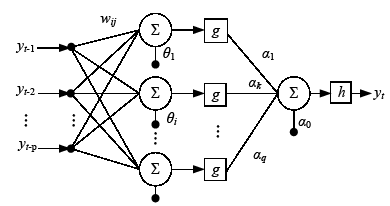
Figure 1.
Time series neural network prediction model
The relationship between output ${{y}_{t}}$ and input $[{{y}_{t-1}}$,${{y}_{t-2}}$,
Here, p is the number of input nodes, q is the number of hidden layer nodes, the parameter ${{\omega }_{ij}}$(i=1, 2,
From the above relation, it can be seen that the above model realizes the nonlinear mapping from the observed samples to the predicted values, i.e.:
Here,w represents all parameters in the above network, and f is determined by the network topology structure and activation function.
2.2. Prediction Steps
The input point of the neural network trend prediction model is the sample value of the time data series of the same state parameter. It is difficult to achieve multi-parameter prediction directly by using this model, so the multi-parameter prediction of the neural network trend model can be considered using the indirect method. First, the data fusion of multiple parameters is carried out using the appropriate statistical analysis method, such as Principal Component Analysis (PCA). The original multiple parameters are simplified into one integrated parameter (main component), and then the trend prediction is carried out with the integrated parameters. The prediction step is shown in Figure 2.
Figure 2
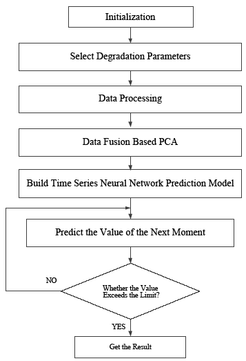
Figure 2.
Steps of neural network trend prediction
After obtaining the sample data of the comprehensive parameter (principal component), the technical condition limit value of the engine is determined, which is measured by the value of the principal component. Then, the neural network trend prediction model is established. The input of the model is the time series data of the main component. With an increase in using time, the main component will tend to decrease or increase. Therefore, when the predicted value of the principal component exceeds its limit value, the prediction is stopped and the final prediction result is obtained.
3. Selecting Degradation Parameters and Data Processing
The test parameters can be determined according to the following three principles [9]: the power and economic performance of the engine can be reflected; it can reflect the change process of the technical state and wear condition of the engine; technically, it can realize the non-disintegration detection of real vehicles. After analysis, the selected test parameters are: cylinder compression pressure ${{\hat{p}}_{\max }}$, fuel supply advance angle ${{\hat{\theta }}_{fd}}$, and vibration energy ${{\hat{V}}_{p}}.$ The tests are performed on a certain type of armored vehicle engine. In this paper, 16 armored vehicles whose engine motor hours are between 0 and 550 hours were selected. The data of these parameters were tested and pretreated, and 16 sample data of three degradation parameters were obtained, as shown in Table 1.
Table 1. Sample data
| Number | Use time/h | ${{\hat{p}}_{\max }}$/MPa | ${{\hat{\theta }}_{fd}}$/ºCA | ${{\hat{V}}_{p}}$/g2 |
|---|---|---|---|---|
| 1 | 11 | 2.8950 | 34.9500 | 54.3540 |
| 2 | 38 | 2.8744 | 33.9796 | 48.7860 |
| 3 | 59 | 2.8647 | 33.9000 | 46.8470 |
| 4 | 103 | 2.8228 | 32.8462 | 42.8991 |
| 5 | 140 | 2.8090 | 32.1142 | 42.0632 |
| 6 | 187 | 2.7958 | 31.1880 | 38.8610 |
| 7 | 190 | 2.7847 | 31.1671 | 36.0951 |
| 8 | 250 | 2.7736 | 31.0942 | 31.3503 |
| 9 | 300 | 2.7521 | 30.3144 | 32.9560 |
| 10 | 320 | 2.7439 | 29.5521 | 32.7874 |
| 11 | 350 | 2.7330 | 29.0114 | 30.8780 |
| 12 | 390 | 2.7132 | 28.9751 | 31.7270 |
| 13 | 450 | 2.6739 | 27.5521 | 28.4621 |
| 14 | 497 | 2.6647 | 26.6285 | 26.5810 |
| 15 | 507 | 2.6527 | 26.4883 | 27.8581 |
| 16 | 550 | 2.6429 | 25.8854 | 25.1580 |
The above parameters influence each other, and their value decreases as the engine’s use time increases. Firstly, the data in the above table should be standardized. According to the requirements of the PCA method [10], the mean value of each parameter’s sample value vector is 0 and the variance is 1, so the following methods are used to standardize the data [11]:
Here, ${{x}_{i}}$ is the characteristic parameter sample value vector, ${{x}_{ij}}$ is the jth sample value of the sample value vector ${{x}_{i}}$, ${{{x}'}_{ij}}$ is the normalized sample value, ${{\bar{x}}_{i}}$ is the mean value of the characteristic parameter sample value vector, and $s$is the standard deviation of the sample vector of characteristic parameters. ${{\bar{x}}_{i}}$ and $s$ could be expressed as:
The data of parameters standardized by the above methods can be seen in Table 4 in the later section.
4. Data Fusion based on Principal Component Analysis
4.1. Principal of PCA
Principal component analysis (PCA) is a multivariate statistical method that uses the idea of dimensionality reduction to transform multiple variables into one or a few comprehensive variables with little information loss. Generally, the transformed comprehensive index is called the principal component, where each principal component is a linear combination of the original variables and each principal component is not related to each other. This makes the principal component have superior performance compared to the original variable. In this way, when studying complex problems, we can only consider a few principal components without losing too much information, so that we can more easily grasp the main contradiction, reveal the regularity between the internal variables of things, simplify the problems, and improve the analysis efficiency [12].
Suppose n samples are collected, and p variables are observed for each sample (x1, x2,
${{X}_{n\times p}}=\left[ \begin{matrix} {{x}_{11}} & {{x}_{12}} & \cdots & {{x}_{1p}} \\ {{x}_{21}} & {{x}_{22}} & \cdots & {{x}_{2p}} \\ \vdots & \vdots & \vdots & \vdots \\ {{x}_{n1}} & {{x}_{n2}} & \cdots & {{x}_{np}} \\ \end{matrix} \right]$
The purpose of principal component analysis is to use p primitive variables (x1, x2,
It can be seen from the above analysis that the essence of principal component analysis is to determine the coefficient lij(i =1, 2,
The practical methods of PCA are as follows:
(1) Standardize original data;
(2) Determine the covariance matrix that is the correlation matrix of the original data from the standardized data. The equation is as follows:
${{R}_{p\times p}}=\left[ \begin{matrix} {{r}_{11}} & {{r}_{12}} & \cdots & {{r}_{1p}} \\ {{r}_{21}} & {{r}_{22}} & \cdots & {{r}_{2p}} \\ \vdots & \vdots & \vdots & \vdots \\ {{r}_{p1}} & {{r}_{p2}} & \cdots & {{r}_{pp}} \\ \end{matrix} \right]$
Here, rij(i, j=1, 2,
(3) Calculate the eigenvalues and the corresponding orthonormal eigenvectors;
(4) Calculate the main component contribution rate (CR) and cumulative contribution rate (CCR);
(5) Determine the number of principal components to be retained.Generally, the main components with a cumulative contribution rate of 85% to 95% are taken.
4.2. Data Fusion
According to the above PCA method, the eigenvalues, variance contribution rate (CR), and cumulative contribution rate (CCR) of parameter correlation coefficient matrix can be obtained, as shown in Table 2.
Table 2. Eigenvalues and variance contribution rate
| Number | Eigenvalue | CR/% | CCR/% |
|---|---|---|---|
| 1 | 2.936 | 97.880 | 97.880 |
| 2 | 0.060 | 1.985 | 99.865 |
| 3 | 0.004 | 0.135 | 100.000 |
Find the length of 1. Mutually orthogonal eigenvectors correspond to the eigenvalues of the correlation coefficient matrix, as shown in Table 3.
Table 3. Eigenvectors
| Parameters | Eigenvectors | ||
|---|---|---|---|
| No.1 | No.2 | No.3 | |
| ${{{\hat{p}}'}_{\max }}$ | 0.581 | -0.333 | -0.743 |
| $\hat{\theta }_{fd}^{'}$ | 0.579 | -0.472 | 0.665 |
| ${{{\hat{V}}'}_{p}}$ | 0.572 | 0.816 | 0.082 |
According to the principle of the PCA method for preserving the number of principal components, it can be seen from Table 2 that the variance contribution rate of only the first eigenvalue is 97.88%. That is, only preserving the first principal component can explain more than 90% of the original parameters. Therefore, the principal component (PC) X can be worked out from the first eigenvector in Table 3 as follows:
The main component data of the parameters are calculated by Equation (10), as shown in Table 4.
Table 4. Standardized data and its principal component
| Number | Use time/h | Standardized data and the PCX | |||
|---|---|---|---|---|---|
| ${{{\hat{p}}'}_{\max }}$ | $\hat{\theta }_{fd}^{'}$ | ${{{\hat{V}}'}_{p}}$ | X | ||
| 1 | 11 | 1.6627 | 1.6318 | 2.1069 | 3.1160 |
| 2 | 38 | 1.4047 | 1.2874 | 1.4641 | 2.3989 |
| 3 | 59 | 1.2832 | 1.2591 | 1.2402 | 2.1840 |
| 4 | 103 | 0.7582 | 0.8850 | 0.7845 | 1.4017 |
| 5 | 140 | 0.5854 | 0.6252 | 0.6880 | 1.0956 |
| 6 | 187 | 0.4200 | 0.2964 | 0.3183 | 0.5977 |
| 7 | 190 | 0.2809 | 0.2890 | -0.0010 | 0.3300 |
| 8 | 250 | 0.1419 | 0.2631 | -0.5488 | -0.0790 |
| 9 | 300 | -0.1275 | -0.0137 | -0.3634 | -0.2898 |
| 10 | 320 | -0.2302 | -0.2843 | -0.3829 | -0.5173 |
| 11 | 350 | -0.3668 | -0.4762 | -0.6033 | -0.8339 |
| 12 | 390 | -0.6148 | -0.4891 | -0.5053 | -0.9294 |
| 13 | 450 | -1.1071 | -0.9942 | -0.8822 | -1.7235 |
| 14 | 497 | -1.2224 | -1.3220 | -1.0994 | -2.1046 |
| 15 | 507 | -1.3727 | -1.3718 | -0.9520 | -2.1364 |
| 16 | 550 | -1.4955 | -1.5858 | -1.2637 | -2.5100 |
5. Establishment of Life Prediction Model
Firstly, the limit value of the principal component is determined as a condition for the prediction cycle to stop. By testing and analyzing the engine close to the overhaul time, the principal component eigenvalues are obtained, as shown in Table 5.
Table 5. The limit value of the principal component
| Number | Use time/h | X |
|---|---|---|
| 1 | 550 | -2.5100 |
| 2 | 550 | -2.5723 |
| 3 | 550 | -2.5510 |
Since the principal component X tends to decrease with the duration of use, the limit of the principal component X takes the maximum value of -2.5100 out of the three values in Table 5 into consideration of the amount of redundancy.
The neural network prediction model generally requires that the input time series data are at equal time intervals, but the engine use time measured in this paper is not equal intervals. Therefore, this paper adopts the interpolation method to get the principal component data at equal time intervals. The time interval cannot be too large, or it may miss important information, so the time interval is taken as 10 hours. The interpolation point data of principal component X is shown in Table 6. The principal component X after equal interval treatment changes with the use of time, as shown in Figure 3.
Table 6. The interpolation point data of principal component X
| Use time/h | X | Use time /h | X | Use time /h | X |
|---|---|---|---|---|---|
| 20 | 2.8770 | 200 | 0.2618 | 380 | -0.9055 |
| 30 | 2.6114 | 210 | 0.1937 | 390 | -0.9294 |
| 40 | 2.3784 | 220 | 0.1255 | 400 | -1.0618 |
| 50 | 2.2761 | 230 | 0.0573 | 410 | -1.1941 |
| 60 | 2.1662 | 240 | -0.0108 | 420 | -1.3264 |
| 70 | 1.9884 | 250 | -0.0790 | 430 | -1.4588 |
| 80 | 1.8106 | 260 | -0.1212 | 440 | -1.5912 |
| 90 | 1.6328 | 270 | -0.1633 | 450 | -1.7235 |
| 100 | 1.4550 | 280 | -0.2055 | 460 | -1.8046 |
| 110 | 1.3438 | 290 | -0.2476 | 470 | -1.8857 |
| 120 | 1.2611 | 300 | -0.2898 | 480 | -1.9668 |
| 130 | 1.1783 | 310 | -0.4036 | 490 | -2.0478 |
| 140 | 1.0956 | 320 | -0.5173 | 500 | -2.1141 |
| 150 | 0.9897 | 330 | -0.6228 | 510 | -2.1625 |
| 160 | 0.8837 | 340 | -0.7284 | 520 | -2.2493 |
| 170 | 0.7778 | 350 | -0.8339 | 530 | -2.3362 |
| 180 | 0.6719 | 360 | -0.8578 | 540 | -2.4231 |
| 190 | 0.3300 | 370 | -0.8817 | 550 | -2.5100 |
Figure 3
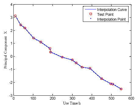
Figure 3.
The interpolation curve of PC X
In this paper, the BP neural network prediction model chooses the hidden layer transfer function as tansig type function and the output layer transfer function as purelin linear transfer function. The neural network is trained by the Levenberg-Marquardt algorithm, and the training error is set as 0.001. The neural network input layer is the interpolation data sequence of the principal component, representing the historical data for prediction. The output is the predicted value, and the output neuron is 1. The establishment of hidden layer nodes is a very important and complicated problem to determine the structure of the neural network model. At present, there is not a theoretically universal determination method. For the trend prediction of neural networks, another important point is the determination of the number of input layer nodes. There is no common theoretical method so far. Both can only be combined with actual experience and through trial and error to find better results and determine the number of input layer and hidden layer nodes[11]. Through trial calculation with Matlab, the input unit of the neural network prediction model is set to 10, and the number of hidden layer neurons is set to 12. The training and prediction effects are improved.
Take the interpolation data of principal component X in Table 6 as the training data of the BP neural network prediction model. The training data is obtained as follows: the first group of input training data takes 10 principal component interpolation points (as a column vector) corresponding to 20-110 motor hours, and the corresponding outputs training data takes the principal component interpolation point corresponding to 120 motor hours; the second group of input training data takes 10 principal component interpolation points (as a column vector) corresponding to 30-120 motor hours, and the corresponding outputs training data takes the principal component interpolation point corresponding to 130 motor hours. By analogy, 44 sets of training data can be constructed to form 10 rows and 44 columns of input matrix, and the corresponding output is a 1 row 44 column output vector. Accordingly, the neural network can be established and trained by Matlab software to determine the weight of the network and establish the life prediction model of the armored vehicle engine. The training error curve can be drawn by Matlab software. It is shown in Figure 4.
Figure 4
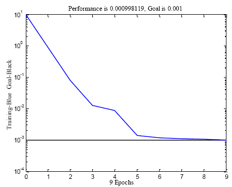
Figure 4.
Training error curve
6. Test and Use of the Model
After establishing the neural network trend prediction model, it is necessary to evaluate the model through testing to ensure that the model can be used after the accuracy requirement is met. In this paper, the mean relative error (MRE) [13] is chosen as the evaluation index of the model, and the required error is not more than 5%. Assume that$x(n)$, (n=1, 2,
The test and use steps of the model are as follows: first, the one interpolation point datum closest to the engine’s use time and its nine previous adjacent interpolation data are used as the first group of input time series data containing 10 data to predict, and the predicted value of the next time interval can be obtained. When predicting the value of the next interval, the predicted value is regarded as the known historical data to be added to the next group of input time series data as the last data value, and the first data value of the input time series data will be removed to keep the input data length unchanged. The simulation is performed step by step. The prediction value of each step will be recorded until the output data reaches the limit value. Then, the predicted value will be compared with the actual interpolation point, and the prediction error can be calculated. The number of simulation steps multiplied by the time interval is the remaining useful life (RUL) of the engine.
In the early stage of engine life, the technical state is generally good. Thus, it is usually not necessary to predict the engine’s life in the early stage. It is only required to predict the life of the engine with a relatively long use time. This paper chooses the engines with a serial number of 9, 10, 11, 12, and 13 (the use time is 300h, 320h, 350h, 390h, and 450h respectively) in Table 4 as the test sample to calculate the model prediction error, while predicting their remaining useful lives.
Figure 5
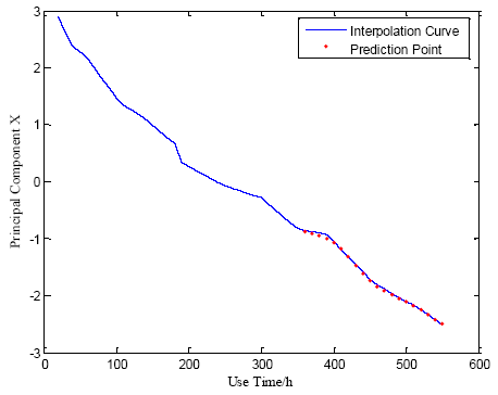
Figure 5.
The prediction results of X
The engines of numbers 9, 10, 12, and 13 in Table 4 are simulated with the same method mentioned above, and their errors and remaining useful lives are calculated. The prediction results are shown in Table 7. It can be seen from Table 7 that the MREis controlled within 4%, satisfying the prediction accuracy requirement. The prediction results of RUL are basically consistent with the actual use life of this type of armored vehicle engine. Furthermore, the data in Table 7 shows that the MRE becomes smaller and smaller as the use time increases. As mentioned before, the engine is usually in good condition in its early period, and it is not necessary to predict its life in this period. In other words, a better and more exact result can be achieved by using this model in the middle or later period of the engine’s life.
Table 7. RUL prediction results
| Number | Use time/h | RUL/h | MRE/% |
|---|---|---|---|
| 9 | 300 | 260 | 4.00 |
| 10 | 320 | 240 | 2.41 |
| 11 | 350 | 200 | 1.57 |
| 12 | 390 | 160 | 1.50 |
| 13 | 450 | 100 | 0.82 |
7. Conclusions
Degradation data provides information about the degradation process, which can be used to analyze the product failure process in depth. The degradation data is of great use value. The useful information in the degradation data can be used to study the reliability of products and indicate a new direction for the reliability technology [14].On the basis of related researches, a model of engine life prediction is constructed using the principal component analysis method and neural network model. Based on the degradation data, the model integrates multiple degradation parameters of the engine into one comprehensive parameter. Then, the interpolation algorithm is used to construct the equal interval time series data of the integrated parameters as the input of the neural network prediction model to predict the remaining life of the engine. The comprehensive parameters can not only comprehensively integrate the various state information of the engine, but also apply to single-parameter neural network forecasting modeling and indirectly realize multi-parameter prediction. The calculation results show that the prediction results are accurate and the model can predict the remaining life of the engine under the actual working conditions after determining the limit technical state. The model is suitable for real-time evaluation and has good application and promotion value.
Armored vehicle diesel engines are complicated and include many systems and parts. It is difficult to get an ideal forecast result with a single method [15]. Conversely, combining several algorithms to make a forecast can not only acquire virtuesbut also remedy respective shortcomings. For example, combining a neural network with fuzzy theory can bring qualitative information under the frame of the neural network. This combination method is better than the single method. It is an inevitable trend to study the combination forecast method [16] in the forecast domain.
Reference
Application of Supportive Vector Machine in Technical States Evaluation of Diesel Engine
,”
Research on Condition based Maintenance for Aero-Engine Using Hidden Markov
,”
Survey of Fault Prognostics Supporting Condition based Maintenance
,”
DOI:10.1631/jzus.2007.A1596
URL
[Cited within: 1]

Some important issues related to fault prognostics including its definition,functionality,algorithmic approaches,difficulties and proposed future work are discussed.By using the curve of system fault degradation,the functionality is introduced.And the recent achievements in the field of fault prognostics according to their different approaches are also reviewed.
Research on Autonomic Logistics Key Technologies for Armored Equipment,” Ph.D. Dissertation,
Review of Reliability Evaluation Technology based on Accelerated Degradation Data
,”
Time Series Prediction based on RBM Neural Network
,”In order to overcome the shortcoming of the dependence on the results of the neural network initialization and the weak generalization,A Neural network based on the restricted Boltzmann Machine(RBM) was presented.Through the unsupervised learning method to optimize the initialization of neural network,the paper integrated the RBM with the neural network.Through experimental comparison with neural network time series prediction model,the result shows that the neural network model based on RBM is better than the pure neural network prediction model,and it can improve the prediction accuracy.
Design of Engine Condition Detection for a Certain Type of Armored Vehicle
,” in
Principal Component and Neural Network Combined Fuel Consumption Forecast
,”
Research on Prediction of Lead-Acid Batteries’ Remaining Discharge Time
”,
Review of Reliability Evaluation Methods based on Performance Degradation Data
,”The reliability evaluation method based on performance degradation data is widely used in the research of high reliable products. Based on it,this paper introduced the research status of performance degradation data reliability evaluation methods. Also the analysis and modeling of degraded data and its application in engineering were introduced. Finally,the exsiting problems were proposed and the prospect of this method was predicted.
Runtime Forecast of Military Vehicle Diesel Engine based on BP Neural Network
,” in
A Survey of Researches on Combination Forecasting Models and Methodologies
,”Prediction accuracy and prediction risk are the core issues of prediction research.From the perspective of complementary information,combination forecasting provides an effective way to improve prediction accuracy.We give a survey of researches on the development of combination forecasting models and methodologies in this paper.We conduct the reviews from several aspects,which are the classification of combination forecasting models,the methods of weight calculation,some kinds of methods of model constructing for combination forecasting. The problems of the optimal sub-models selection in the combination forecasting are reviewed and discussed,and finally we give the prospects and future research directions of combination forecast models under uncertain environment.
