Design and Study of Performance Characteristics of Flat Wall Rectilinear 3D Diffuser with Square Inlet and Rectangular Outlet
Kumar Manish
通讯作者:
版权声明: 2020 Totem Publisher, Inc. All rights reserved.
展开
Abstract
The present study explores the design of a flat wall rectilinear 3D diffuser with square inlet and a rectangular outlet for subsonic, incompressible flow. In this 3D diffuser, the diffuser walls are diverged in the horizontal plane to control the flow separation from the walls of the diffuser, which results in a decrease in the coefficient of static pressure recovery; this is a phenomenon called ‘stall’. In case of a wide angled 2D diffuser, 'stall' is a serious issue. In present work, a 3D diffuser was designed with the same area ratio (4), aspect ratio (1), and non-dimensional length (8.21) as those of a 2D diffuser. With varying Reynolds numbers, it was found that the coefficient of static pressure recovery increases continuously for the 3D diffuser. In case of the 2D diffuser, it decreases as the Reynolds number exceeds 2×10⁵. From CFD analysis, it was found that vectors lie in the mid-longitudinal plane. A three-hole probe was used to measure local velocity to achieve velocity profiles at five different -2 equally distant planes between the inlet and outlet. The maximum error in the experimental results and that of the CFD analysis for the velocity profile and coefficient of static pressure recovery were 9% and 1.02%, respectively.
Keywords:
© 2020 Totem Publisher, Inc. All rights reserved.
1.Introduction
In internal flow systems, diffusers are used to convert kinetic energy into pressure energy by decelerating the flow in the direction of fluid motion. A diffuser is an essential component of turbomachinery, including turbines, combustors, steam turbine exhaust hoods, flow meters, intake of modern aircraft engines, injectors, draft tubes for hydraulic turbines, wind tunnels, and ventilation ducts. Though the geometry of a diffuser appears simple, the flow inside the diffuser is complicated. When hydraulic turbines were developed, the goal was to increase the expansion ratio to obtain more power, but as a result, the pressure at exit fell below the atmospheric pressure. To avoid this problem, the draft tube was used to exhaust water to the tailrace. From then on, the diffuser came into existence. A basic feature of a diffuser is to increase the static pressure head by converting the kinetic energy of fluid into potential energy. In past performance data and flow characteristics of subsonic flow, the straight centre line two-dimensional diffuser is investigated, in which flow regimes as a function of overall diffuser geometry is determined [1-2]. The separation or stall from the diffuser wall affects the performance of the diffuser. The separation is responsible for a lower pressure recovery. A stall can be prevented or controlled by optimizing geometrical parameters like angle of divergence and non-dimensional length. At a non-dimensional length of 1.5, the allowable angle of divergence should be less than or equal to 2 degrees. In order to obtain optimum pressure recovery, geometrical parameters must be within certain limits [3]. A correlation between a 2D straight flat wall diffuser and conical diffuser by aspect ratio and area ratio is estimated. The correlation between flow regime data between flat wall 2D geometry diffusers and that for a conical diffuser is also investigated with the assumption of reasonable inlet conditions and low Mach number. It was found that for the same area ratio and aspect ratio, there exists an appreciable stall for a conical diffuser and transitory stall for a 2D flat wall diffuser [3]. Hence, for the same non-dimensional length and aspect ratio, the probability of stall is more in a 2D flat wall diffuser than in a conical diffuser. For flow-through diverging ducts, the angle of divergence should be in the range of 20-160 in case of diffusers, and the non-dimensional length should be in the range of 1.5-20 to avoid separation [4]. The prediction of stall for 2D flat wall diffusers depends not only on geometrical parameters limits but also on pressure distribution on the walls [5]. For subsonic flow, a free stream boundary layer is not sufficient to describe the solution at a particular point. If boundary layer is assumed to be parabolic, it provides not only the solution but also the point of separation. Radial diffusers are frequently used in turbomachines to achieve appreciable static pressure recovery without increasing the length of the diffuser. In a radial diffuser, fluid flows radially outward in a confined space between two boundaries and remains in the meridional plane. Like the axial flow diffuser, numerous investigations on radial diffusers have been carried out on varying several geometrical parameters like passage width, radius ratio, wall shape, and number and geometry of vanes, and these are well documented in the literature [6-7]. S-shaped and Y-shaped diffusers are studied by [8] and [9], respectively, while the performance of hybrid diffusers is studied by [10]. Research is still ongoing, and many radial diffusers such as pipe diffusers and inland diffusers are emerging.
In the case of design of diffusers, there are certain parameters that are very important. Aerodynamic parameters play a great role in the performance of the diffusers. In the past, these were ignored, but with the time, the existence of these parameters became very important in predicting the performance of diffusers precisely. These parameters depend on the type of diffusers. Aerodynamic blockage signifies how much core area is reduced due to the formation of the boundary layer. It is the function of boundary layer displacement thickness. As the flow takes place in the diffuser, the boundary layer thickness continuously increases in the direction of flow. Hence, the effective core area in the direction of flow continuously decreases. Viscosity is a very important parameter in any fluid dynamics system process and normally appears in the form of the Reynolds number. Typically, diffusers are characterized by Reynolds number based upon hydraulic diameter. The inlet Mach number defines the compressibility of the fluid. If the Mach number is less than 0.3, i.e., U = 102m/s, the flow will be incompressible. Turbulent intensity is more frequently is defined as the ratio of RMS value of turbulent kinetic energy per unit mass to mean velocity of flow. Alternatively, it can also be defined as a function of hydraulic diameter. Swirling flow into the inlet of diffuser implies that there is a component of velocity in the tangential direction as the flow enters the diffuser. This effect has been considered most often for conical and annular diffusers but probably is relevant also for channel diffusers as employed in various pumps and compressors. The coefficient of static pressure recovery is the measure of static pressure recovery, which is defined as a rise in static pressure head to dynamic head at the inlet. Velocity profile measurements in the diffuser inlet showed that the streamwise vortices affect the uniformity of the streamwise mean velocity, accounting for some of the performance changes [11].
2.Methodology
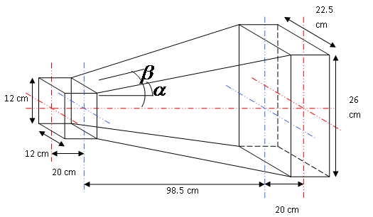
In this study, velocity profiles and velocity vectors at five equally distant planes and the coefficient of static pressure recovery are found along the length of the diffuser with the help of CFD code (FLUENT). Results obtained are validated experimentally. The present work depends on 3D geometry, a flat wall rectilinear diffuser with square inlet, and a rectangular outlet. To avoid separation, the total angle of divergence should not exceed 16°. So, for an area ratio of 4, various combinations are made for α and ß, which are respectively the semi angle of divergence in transverse plane and longitudinal plane such that α ≠ ß and 2° ≤ α ≤ 8°. Thus, the non-dimensional length L/a0 is calculated for all possible combinations of α and ß (in the permissible range). After that, for a particular value of L/a0 (within the permissible range) and the corresponding value of α and ß, the formed geometry of the current problem must be simulated for steady, subsonic, 3D, and incompressible flow.
From the Bernoulli equation:
From the continuity equation:
Let
a0 = Side of square at inlet, L = length of diffuser, and L/a0 = non-dimensional length
a1 = Height of rectangular exit of diffuser
a2 = Width of rectangular exit of diffuser
The non-dimensional length L/a0 is chosen as 8.21, which corresponds to α = 4° and β = 3°. According to these design parameters, the corresponding values of geometric dimensions of L, a0, a1, a2 are calculated as 98.5, 12, 20, and 12.5cm, respectively. Hence, the 3D designed diffuser is shown in Figure 1 below.
3. CFD Analysis
The CFD code (FLUENT) using the standard k-ε model was used to draw velocity vectors at the exit of the diffuser and central longitudinal velocity profiles at five equally distant planes from the inlet. FLUENT was used with two equations using the standard k-ε model.
Solution criteria: (Governing equations, relaxation factors, pressure velocity coupling, discretization)
Equation of turbulence: (Nevier Stoke's equation)
Equation of flow: (Continuity equation)
Constant values for the standard
The fluid properties of air at S.T.P are given in Table 2.
Table 2 Properties of air at S.T.P.
| Density of air ( | Dynamic viscosity ( |
|---|---|
| 1.225 | 1.7894e-5 |
The relaxation factors for various parameters are given in Table 3.
The solution limits for minimum and maximum absolute pressure, minimum k, minimum
Table 4 Solution limits for minimum and maximum absolute pressure, min. k, min , and max.
| Minimum absolute pressure | Maximum absolute pressure | Min. k | Min. | Max. |
|---|---|---|---|---|
| 1 (Pa) | 5e+10 (Pa) | 1e-14 | 1e-20 | 100,000 |
A meshed diffuser with hexahedral cells and a boundary layer at inlet and outlet is shown in Figure 2.
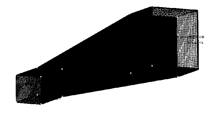
Figure 2. Designed diffuser with boundary conditions: mean velocity of flow at inlet and gauge pressure at outlet is zero
Figure 3 shows contours of velocity and vectors at the exit of the diffuser.
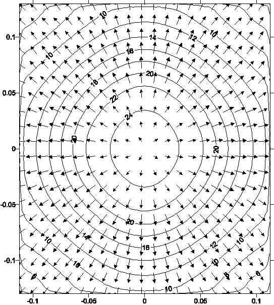
Similar velocity vectors lie in the longitudinal plane from plane no. 1 to plane no. 5.
4.Experimental Setup
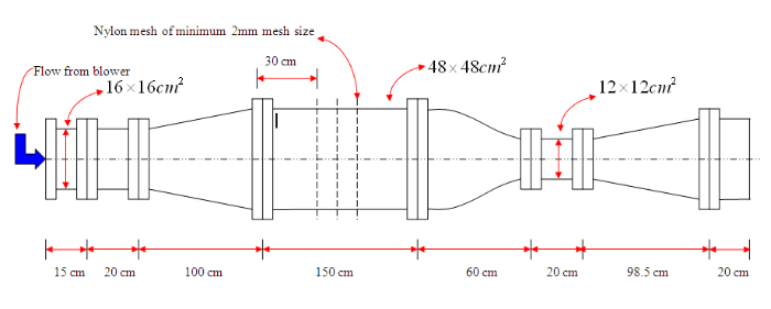
Apparatus and equipment used: Glass tube water manometer, three-hole probe pitot tube, Betz micrometre, pitot static tube, traversing mechanism (with longitudinal, transverse, and vertical movement), designed test rig, calibration tunnel, thermometer, and barometer. The block diagram of the experimental setup is shown in Figure 4.
Fluid(air, water) properties at atmospheric conditions are mentioned in Table 5 given below.
Table 5 Fluid properties at atmospheric conditions
| Temperature | t = 36 |
|---|---|
| Atmospheric pressure | 73.3cm of Hg = 97793.928Pa |
| Density of air at 36 degree Celsius | |
| Density of water at 36 degree Celsius |
Through CFD analysis, it was observed that the velocity vectors also lie in the plane of the central longitudinal plane of the diffuser. Thus, a three-hole probe was used to experimentally validate the velocity profiles for those equally distant planes. To measure the mean velocity, a flow pitot static tube was used. In the experimental setup, the static pressure at the wall of the diffuser was measured using metallic static tubes. Figure 5 shows the experimental setup for calibration of the three-hole probe.
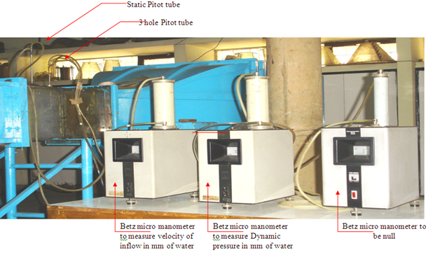
Figure 5. Experimental setup for calibrating three-hole probe in a subsonic low turbulence wind tunnel
In the null position
Readings obtained by the above experimental setup and calculations are given in Table 6.
Table 6 Readings taken for calibrating three-hole probe
| i | Average static pressure in mm of the inclined water column | Average static pressure in mm of the vertical water column | % | ||
|---|---|---|---|---|---|
| 1 | 0.5781 | -22.00 | -19.13 | -187.01 | 75.29 |
| 2 | 0.6624 | -17.25 | -15.07 | -147.27 | 79.67 |
| 3 | 0.7468 | -14.00 | -12.18 | -118.98 | 82.77 |
| 4 | 0.8312 | -11.25 | -9.77 | -95.49 | 85.29 |
| 5 | 0.9156 | -9.50 | -8.17 | -79.84 | 87.03 |
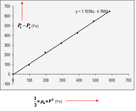
From the above readings, the value of the calibrating constant, which is a multiple of x, of the generated equation is obtained by the graph. It is shown in Figure 7.
5. Results and Discussion
5.1. Comparison of Performance 3D Geometry Diffuser with of 2D Geometry Diffuser for Same Geometrical Parameters
The variation of mass averaged static pressure recovery with respect to Reynolds number at inlet is given in a self explanatory Figure 8 for both 2D and 3D geometry diffuser.
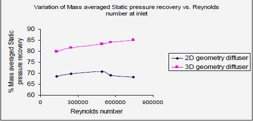
Figure 8. Variation of mass averaged static pressure recovery vs. Reynolds number
5.2. Validation of Velocity Profiles
For the validation of longitudinal velocity, five equally distant planes were taken from the diffuser exit as shown in Figure 9.
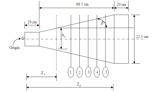
Since 'O' is the global coordinate at the inlet, we measured all the distances from 'O'. Let (ZL = 118.5) be the coordinate of the end of the diffusing section from the origin.
For the ith plane, the width of the diffusing section at coordinate Zi can be defined as:
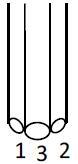
Five holes were taken at each plane at equal distances, and they were numbered as
In the experimental setup, the angle of inclination is kept as Ө = 30°.
Vertical height of water column = (3)0.5/2
Vertical height of water column = 0.87
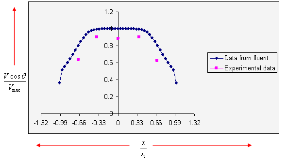
5.2.1. Validation of Central Longitudinal Velocity Profiles for Inlet Mean Velocity = 40m/s
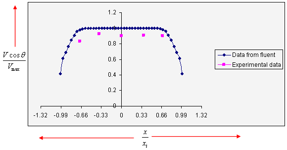
For plane no. 1, the validation of velocity profiles is shown in Figure 10.
-0.08585 ≤ x1 ≤ 0.08585, y = 0, and Zi/ZL = 0.5781. The fluent longitudinal velocity component Vmax = 23.26m/s.
For plane no. 2, the validation of velocity profiles is shown in Figure 11.
-0.09115 ≤ x2 ≤ 0.08585, y = 0, and Zi/ZL = 0.6624. The fluent longitudinal velocity component Vmax = 23.26m/s.
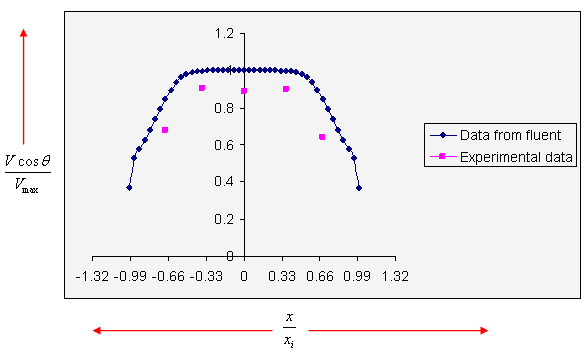
For plane no. 3, the validation of velocity profiles is shown in Figure 12.
-0.0965 ≤ x3 ≤ 0.0965), y = 0, and Zi/ZL = 0.7468. The fluent longitudinal velocity component Vmax = 20.50m/s.
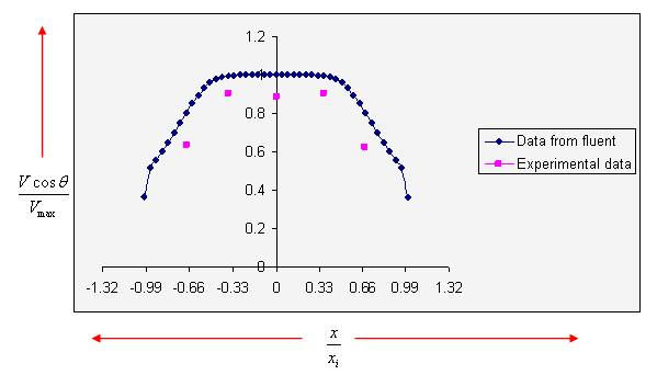
For plane no. 4, the validation of velocity profiles is shown in Figure 13.
-0.10185 ≤ x4 ≤ 0.10185), y = 0, and Zi/ZL = 0.8312. The fluent longitudinal velocity component Vmax = 19.51m/s.
For plane no. 5, the validation of velocity profiles is shown in Figure 14.
-0.10715 ≤ x5 ≤ 0.10715), y = 0, and Zi/ZL = 0.9165. The fluent longitudinal velocity component Vmax = 18.72m/s.

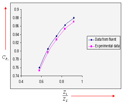
5.2.2. Experimental Validation for Static Pressure Recovery in the Direction of Flow for Inlet Mean Velocity U = 40m/s as Obtained from FLUENT
Velocity at inlet, i.e., at Z= 0, U =40m/s.
Mass averaged Static pressure at inlet, i.e., at Z = 0, Pst0 = -871.08Pa.
For the glass tube water manometer, the average static pressure at Z= 0.04 m, is 92.75mm of the vertical water column sub atmospheric i.e. -906.37Pa.
Readings obtained from the inclined glass tube manometer for static pressure in terms of the water column and corresponding pressure at different coordinates and mass averaged coefficients of static pressure recovery are given in Table 7.
From Figure 15, it is clear that in the case of the 3D flat wall diffuser, the coefficient of static pressure recovery increases gradually as the Reynolds number increases. For the 2D flat wall diffuser, stall occurs when the Reynolds number exceeds 2
The maximum error in the experimental data for velocity profiles = 9%.
The maximum error in the experimental data for static pressure recovery = 1.02%.
Table 7 Data for validation of static pressure recovery for U = 40 m/s
| I | Average static pressure in mm of inclined water column | Average static pressure in mm of vertical water column | % | ||
|---|---|---|---|---|---|
| 1 | 0.5781 | -22.00 | -19.13 | -187.01 | 75.29 |
| 2 | 0.6624 | -17.25 | -15.07 | -147.27 | 79.67 |
| 3 | 0.7468 | -14.00 | -12.18 | -118.98 | 82.77 |
| 4 | 0.8312 | -11.25 | -9.77 | -95.49 | 85.29 |
| 5 | 0.9156 | -9.50 | -8.17 | -79.84 | 87.03 |
6.Conclusion
It can be concluded that the 3D geometry diffuser provides higher static pressure recovery than the 2D geometry diffuser for the same geometrical parameters within the permissible limit, same inlet velocity, and same hydraulic diameter. However, the increment in static pressure recovery for the 3D geometry diffuser at the inlet straight portion decreases due to core flow, and after that, the static pressure coefficient increases continuously. For the designed diffuser using CFD analysis and further experimental validation, it can be concluded by the velocity profiles that the turbulent flow inside the diffuser develops uniformly because the flow is kept subsonic. As mean velocity at the inlet increases, turbulent flow inside the diffuser increases, which results in lower static pressure recovery because of higher turbulence intensity.
The presently designed 3D geometry diffuser can be used without separation, where space is limited for the same pressure recovery as that for a 2D geometry diffuser. It can also be used when we need to connect a square-sectioned duct to a rectangular duct of larger hydraulic diameter.
The authors have declared that no competing interests exist.
参考文献
| [1.] |
“Performance and Design of Straight Two-Dimensional Diffuser,” Journal of Basic Engineering, Vol. 89, No .
|
| [2.] |
Reneau and J. P. Johnston, “A Performance Prediction Method for Unstalled Two Dimensional,” Journal of Basic Engineering, Vol .
|
| [3.] |
“Optimum Design of Straight-Walled Diffuser,” Journal of Basic Engineering, pp. 321-331,
|
| [4.] |
“Internal Flow System,” 2nd Edition, BHRA Publications,
|
| [5.] |
Moses and J. R. Chappell, “Turbulent Boundary Layers in Diffusers Exhibiting Partial Stall,”
|
| [6.] |
“Research on Optimizing Design for Diffuser-Tower Structure of Primary Fan in Shaft,” New Trends in Fluid Mechanics Research, Springer, Berlin,
|
| [7.] |
|
| [8.] |
|
| [9.] |
|
| [10.] |
|
| [11.] |
|

/
| 〈 |
|
〉 |