Operational readiness is one of the most important indexes of operational capability and the overall index for the effectiveness of the equipment support system of system (SoS). A scientific and reasonable assessment model is of great significance for optimizing the structure of the support SoS and improving the effectiveness of the support SoS. Aiming at the problem of inadequate consideration of the support factors in the existing assessment model, a new assessment model of the operational readiness rate that considers a variety of support factors is proposed. From the perspective of equipment support mission requirements, the equipment readiness assessment models for a single combat unit and multiple combat units are constructed. Finally, the accuracy of the proposed model is verified by an example analysis and comparison, and the influence of different support factors on the operational readiness rate is quantitatively analyzed.
Keywords: operational readiness rate;
two-level support SoS;
support factors
Long Gao. Assessment Model for Operational Readiness Rate of Equipment System of System under Two-Level Support System. [J], 2019, 15(2): 485-496 doi:10.23940/ijpe.19.02.p13.485496
Nomenclature
SoS–System of system
$L$–Number of the type of support requirements
${{n}_{l}}$–Number of the lth type of support requirements, $1\le l\le L$
${{T}_{s}}$–Time length of the operation preparation phase
${{T}_{l}}$–Completion time of the lth type of support requirements
${{T}_{i}}$–Completion time of theith support stage
${{\lambda }_{i}}$–Parameter of ${{T}_{i}}$ with exponential distribution
${{p}_{i}}$–Probability that the support requirements can be dealt with successfully
${{P}_{e}}\left( {{T}_{s}} \right)$–Operational readiness rate at the beginning time ${{T}_{s}}$
1. Introduction
Operational readiness refers to the ability that the equipment can start performing scheduled tasks at any time when it receives a combat or training command. It reflects the ability that the equipment can be sent out to conduct operations at a specific time node[1]. It is the result of comprehensive action of equipment reliability and maintainability, support system characteristics and capabilities, troops training, and other factors. The typical parameters of operational readiness have the operational readiness rate, availability, and executable task rate. The operational readiness rate is the probability measure of operational readiness, which indicates the probability that the equipment is ready to execute the mission when required to be put into combat or training.
The definition and factors of operational readiness and the typical assessment model of operational readiness rate were summarized in references [2-3]. Rodrigues et al. [4] used simulation methods to study how to improve the operational readiness of the A-4 aircraft through joint support. Zhang et al. [5] presented an assessment model of readiness rate of complex weapon systems during the mission preparation phase under the condition that mission start requirements, the states at mission notification moments, and the maintenance support plan were known. Liu et al.[6] proposed an assessment model of the fleet readiness rate under the condition of given fleet states during the mission preparation period and established the relationship between maintenance support capability and fleet operational readiness rate. Ding et al. [7] proposed a new type model of operational readiness rate that considers maintenance support and spare parts support simultaneously. Wei et al. [8] established a mission-based readiness assessment model in the case that the reliability, maintainability, supportability, and maintenance process of the naval gun equipment were considered. Han et al. [9] gave a fleet readiness assessment model based on the Markov model. Ding et al. [10] proposed a readiness assessment model based on the spare part delay time model of two-stations and three-stations, which was expressed by the RMS parameters of LRU. Dong et al. [11] studied the operational readiness rate model torpedo inventory with a LRU failure, multiple identical LRU failures, and multiple different LRU failures. According to the actual support condition during the missile service, the evaluation method and model of the readiness rate of missile equipment based on the diffusion process were given in reference [12]. A three-level support assessment model of spare parts was established based on the METRIC theory, and the indexes of the support degree of support SoS were put forward according to the readiness rate of operational unit equipment in reference [13]. Ruan et al. [14] proposed a mission-driven simulation model for the fleet operational readiness and obtained a curve of readiness rate to support time by means of the PERT network method with determined logic but random duration and the Monte Carlo. The multi-level coordination optimization allocation model of operational readiness was established in reference [15], and it was suitable for the design and development of large-scale weapon equipment.
Overall, the assessment of operational readiness rate involves the three aspects of operational missions, the equipment itself, and the support ofSoS. Due to different research priorities and perspectives, a variety of assessment models have been presented successively to apply to different situations. However, these models still have some shortcomings: 1) the existing assessment models pay more attention to maintenance support work but rarely consider the supply support work simultaneously.Only the model proposed in reference [7] considers both maintenance support and supply support of spare parts, but the model is only applicable to single equipment or equipment groups with multiple identical equipment; 2) the existing model mainly focuses on the readiness assessment during the mission period, and it does not apply to the missions in which the equipment is difficult or impossible to support. Only the model mentioned in the reference [6] is usable, but it requires the number of failed LRU to keep with the the number of failed equipment; 4) the existing methods to establish the assessment model are based on the basic maintenance level agreement, namely LRU and SRU, but they will face the combinatorial explosion problem when they are used to deal with the equipment SoS and to support SoS with more complex structures and behaviour.
Therefore, this paper begins from the perspective of equipment support requirements and then establishes a new assessment model of operational readiness rate in the case that it is difficult or impossible to support during the mission execution and the mission requirements, structure, and states are known. This model takes into account a variety of support factors including maintenance support and supply support. Finally, the model is verified by an example and the influence of the different support factors on readiness rate is studied quantitatively.
2. Problem Description
The equipment SoS refers to a higher-level complex system composed of various weapons equipment that are functionally interconnected and interacting under the conditions of strategic guidance, operational command, and support, which is in order to complete certain missions[16]. According to the current institution and establishment of the military, the equipment collection of the combat unit belonging to a certain military services can also be regarded as an equipment SoS. The combat unit is usually composed of a battle unit with combat capability and a basic support unit that is not capable of fighting but is responsible for supporting the combat unit. The basic support unit is a basic combination consisting of a certain number of support personnel and support resources, which has certain supportability, such as a repair team, rescue unit, equipment support unit, and so on. The support unit is a support entity with relatively high supportability that is composed of a plurality of basic support units and can carry out various different support tasks. Both the support unit and the combat unit are equipped with the ability of spare parts inventory, fault parts maintenance, and supply support.
The relationship between the equipment SoS composed of a plurality of combat units and the support SoS composed of a plurality of support units is shown in Figure 1, in which the support units and the basic support units that belong to the combat units constitute a two-level support organization.
Figure 1.
Relationship between the equipment SoS and two-level support organization
During the combat or training tasks, each combat unit in the equipment SoS will generate different equipment support requirements due to factors such as fire strikes of the enemy, component wear, and human errors. The corresponding task objectives of different support requirements are different, and the support unit and support resources required are also different. There are also differences in the completion location of tasks, execution time, and number of equipment. These will affect the decomposition of support tasks and support subtasks, and the decomposition process is shown in Figure 2.
Figure 2.
Decomposition process of the support requirements to support tasks
The equipment support requirements generated by different combat units can be divided into different support tasks according to the different contents of the tasks. For example, the support requirements of a typical task can be decomposed into the use support tasks, maintenance support tasks, and supply support tasks. According to the principle of equipment support task decomposition, each support task can be further decomposed and eventually refined into meta-tasks. The set of all meta-tasks constitutes a meta-task library. In the support task space, each task has its corresponding meta-task. The meta-task is the basic task that can no longer be decomposed in the equipment support task space. In the support task space, each task has its corresponding meta-tasks.
The support process of the equipment SoS is shown in Figure 3. The support requirements will be positioned and evaluated when the combat units in the equipment SoS produce equipment support requirements. If the basic support unit can meet the support requirements, the support task will be completed in the basic support unit, and the support resources that can be used repeatedly are sent to the warehouse of this unit as reserve resources. If the basic support unit cannot meet the support requirements, the support requirements will be transferred to the support unit that can perform multiple support tasks simultaneously to deal, and the corresponding support resources will be applied from the resource warehouse of this unit. Compared with the basic support units, the support units generally have a relatively larger supportability and can meet and complete the support requirements with high probability. The reusable support resources can be sent to the warehouse of this unit as reserve resources. If the resources needed by support requirements are consumable resources, then these resources involved will exit the support organization.
Based on the above analysis, it can be seen that the operational readiness rate of the equipment SoS is related to factors such as the equipment states at the end of the current mission, support system structure, number and supportability of the support units, satisfaction rate of the support resources, speed of supply support, and so on. If the combat unit does not have the support requirements before performing the mission, it can be immediately put into operation or use. If the combat unit has generated equipment support requirements before performing the mission, but its support time is less than the time required to re-enter combat or use, it indicates that there is enough time for providing support to invest in the next battle or use. For the missions that are difficult or impossible to support during the execution period, the support work during the interval between the end of the current mission and the start of the next mission will have an important effect on the outcome of the next mission.
3. Assessment Model Establishment
3.1. Basic Assumptions
· Equipment that is in well readiness condition at the time of mission notification will not generate equipment support requirements during the mission preparation phase;
· The supply speed of support resources is basically fixed, and the time to delay in the supply support are only related to the distances;
· Occupancy-type support resources are always in the idle state;
· The time to apply and deal with application of resources is subordinate to the general distribution;
· The completion time of all support subtasks obeys the exponential distribution.
3.2. Assessment Model of Operational Readiness Rate for a Single Combat Unit
Assume that the equipment belonging to a certain combat unit in the equipment SoS may generate $L$type of support requirements, and the requirement number of this type is ${{n}_{l}}$ in this unit. The time to apply and deal with the application of resources of all support requirements are subject to the general distribution with the probability density function $g\left( t \right)$. The average distance for obtaining support resources is $\bar{s}$, the average speed for supply resources is $\bar{v}$, and then the probability of obtaining the required consumptive support resources in the mission preparation phase is calculated by
Where ${{T}_{s}}$ is the time length of the operation preparation phase; the form of the function $g\left( t \right)$ can be determined by the formation of the delay time that the grassroots force spends on obtaining the support resources.
The completion time of the${{l}^{\text{th}}}$type of support requirements is ${{T}^{l}}$, and the conducting process of this requirement is divided into $r$ phases.
The conducting time ${{T}_{i}}$ of the ${{i}^{\text{th}}}$, ($1\le i\le r$)support phase is subordinate to the exponential distribution with ${{\lambda }_{i}}$, the probability that this requirement can be successfully handled in this phase is ${{p}_{i}}$, and the process that support requirements are handled by stages is shown in Figure 4.
When all support phases cannot successfully handle the support requirement, the completion time of this requirement is the sum of the processing time in all support phases. The probability is calculated by
When the support requirement is successfully completed in the ${{k}^{\text{th}}}$phase, the completion time ofthis requirements is the sum of the processing time in the previous $k-1$support phase. The probability is calculated by
hus, the process of support requirement obeys the Cox distribution. The Cox distribution is actually composed of a number of mutually independent exponential distributions. According to the Laplace transform of the Cox distribution [17], the Laplace expansion of the time distribution of support requirements is
$\hat{F}\left( s \right)=\sum\limits_{i=1}^{r}{\prod\limits_{j=1}^{i}{\left( 1-{{p}_{j-1}} \right){{p}_{j}}\frac{{{\lambda }_{j}}}{{{\lambda }_{j}}+s}}}$
The Laplace transform of completion time distribution of support requirementsis rationalized, and then the inverse Laplace transform can be used to obtain the density function ${{f}_{1}}\left( t \right)$ of that completion time distribution of support requirements. This paper mainly considers the two-level equipment support system consisting of the support unit and the basic unit belonging to combat. The basic support units and support units will handle the support requirements successively. The process of support requirement handling mainly includes two phases: the basic support unit processing phase and the superior support unit processing phase. At this time, the probability density function ${{f}_{1}}\left( t \right)$ of the completion time distribution of support requirements is as follows:
Where ${{p}_{1}}$ is the probability that the basic support units belonging to the combat unit can successfully complete the support requirements, and${{\lambda }_{1}}$and${{\lambda }_{2}}$ are the exponential distribution parameters of the processing time of the basic support unit and the superior support unit, respectively.
Assume that the equipment in the combat unit at the time of mission notification is in an incomplete state due to the presence of the ${{l}^{\text{th}}}$ type of support requirements, the support resources required by this requirement are missing, and the mission start time ${{T}_{s}}$ is given. Then, the probability that this support requirement can be successfully completed at the beginning of the operation mission is
$P_{t}^{l}=P\left( {{T}^{l}}\le {{T}_{s}} \right)=\int\limits_{0}^{{{T}_{s}}}{{{f}_{1}}\left( t \right)\text{d}t}$
Thus, the operational readiness rate of the individual combat units in the equipment SoS at the beginning time ${{T}_{s}}$of the mission can be calculated by
Where $P_{c}^{l}={{{n}_{l}}{{\lambda }_{l}}}/{\sum\limits_{l=1}^{L}{{{n}_{l}}{{\lambda }_{l}}}}\;$ indicates the probability that the equipment of combat unit is in an incomplete condition due to the generation of the${{l}^{\text{th}}}$ type support requirement, and${{P}_{0}}$ indicates the probability that the equipment of combat unit is in a readiness condition at the end time of the current mission.
3.3. Assessment Model of Operational Readiness Rate for Multiple Combat Units
In the context of informatization joint operations, the equipment SoS for conducting combat missions generally contains multiple combat units. Each combat unit cooperates with each other to complete missions. In this process, the equipment support SoSthat can carry out multiple support tasks provides support at the same time. Therefore, we need to study the operational readiness rate assessment model for multiple combat units under sharing the equipment support SoS.
Assume that the equipment SoS conducting combat missions consists of $M$combat units, and the number of combat units with support requirements at the time of mission notification is $m$, in which the number of the type of support requirements is $L$. When $m=1$, the readiness assessment model for multiple combat units is the same as the single combat unit. Therefore, here we will focus on the operational readiness rate at the beginning moment of the next mission under the condition that there are $m>1$combat units needed to be supported at the notification moment of mission.
At the notification moment of mission, there are ${{m}_{1}}$ units, which, due to support requirements, cannot be completed in basic support. There are ${{m}_{2}}$ units, which, due to support requirements, can be completed in basic support in $m$combat units generating support requirements, and $m={{m}_{1}}+{{m}_{2}}$. Then, the operational readiness rate of the $m$ combat units is the probability that the acquisition time of the support resources of the ${{m}_{1}}$ combat units and the completion time of the support tasks of ${{m}_{2}}$are less than the mission start time ${{T}_{s}}$. For ${{m}_{1}}$ combat units with support requirements, the probability that the acquisition time of support resources is less than ${{T}_{s}}$ can be obtained according to Formula (1). For ${{m}_{2}}>1$combat units with support requirements, there are two situations in which support requirements are the same or not. Therefore, the situation that ${{m}_{2}}$ combat units are caused by the same support requirements is first given.
Assume that ${{m}_{2}}$ combat units are caused by ${{n}^{l}}\left( {{m}_{2}} \right)=\sum\limits_{i=1}^{{{m}_{2}}}{n_{i}^{l}}$ support requirements of the${{l}^{\text{th}}}$type , where $n_{i}^{l}$ is the number of support requirements of the ${{l}^{\text{th}}}$ type in the${{i}^{\text{th}}}$combat unit. The completing time of${{l}^{\text{th}}}$ typesupport requirements is subject to independent and identical distribution ${{F}_{l}}\left( t \right)$. The number of support unit is $c$. When $1<{{n}^{l}}\left( {{m}_{2}} \right)\le c$, the completion time of ${{n}^{l}}\left( {{m}_{2}} \right)$ support requirements of the${{l}^{\text{th}}}$type is
Where $T_{i}^{(l)}$ indicates the completion time of the${{i}^{\text{th}}},$ ($1\le i\le {{m}_{2}}$) support requirements of the${{l}^{\text{th}}}$ type. Then, the distribution ${{T}^{\left( {{n}^{l}}\left( {{m}_{2}} \right),l \right)}}$ can be calculated by
$\begin{matrix} & {{F}_{{{m}_{2}},l}}\left( t \right)=P\left( {{T}^{\left( {{n}^{l}}\left( {{m}_{2}} \right),l \right)}}\le t \right)=P\left( \max \left\{ T_{1}^{(l)},T_{2}^{(l)},\cdots ,T_{{{n}^{l}}\left( {{m}_{2}} \right)}^{(l)} \right\}\le t \right) \\ & =\prod\limits_{i=1}^{{{n}^{l}}\left( {{m}_{2}} \right)}{P\left( T_{i}^{\left( l \right)}\le t \right)}={{F}_{l}}{{\left( t \right)}^{{{n}^{l}}\left( {{m}_{2}} \right)}} \end{matrix}$
Where${{F}_{l}}{{\left( t \right)}^{{{n}^{l}}\left( {{m}_{2}} \right)}}$ indicates the power ${{n}^{l}}\left( {{m}_{2}} \right)$of distribution${{F}_{l}}\left( t \right)$.
When ${{m}_{2}}>c$, assume that ${{\theta }_{i}}$ ($1\le {{\theta }_{i}}\le {{n}^{l}}\left( {{m}_{2}} \right)$) is the number of support requirements completed by the support unit $i$ ($1\le i\le c$) in the ${{T}^{\left( {{n}^{l}}\left( {{m}_{2}} \right),l \right)}}$, ${{n}^{l}}\left( {{m}_{2}} \right)=\sum\limits_{i=1}^{c}{{{\theta }_{i}}}$,and $T_{{{\theta }_{i}}}^{(l)}$is the time to complete the ${{\theta }_{i}}^{\text{th}}$support requirement. Then, there is
Since the process of fulfilling support requirements for each support unit is an update process, the distribution of ${{T}^{\left( {{n}^{l}}\left( {{m}_{2}} \right),l \right)}}$ can be calculated by
Where $F_{l}^{\theta _{i}^{*}}\left( t \right)$ represents the ${{\theta }_{i}}$ re-convolution of the distribution function ${{F}_{l}}\left( t \right)$, and${{S}_{{{n}^{l}}\left( {{m}_{2}} \right)}}$ represents all possible combinations $\left( {{\theta }_{1}},{{\theta }_{2}},\cdots ,{{\theta }_{c}} \right)$ that satisfy${{n}^{l}}\left( {{m}_{2}} \right)=\sum\limits_{i=1}^{c}{{{\theta }_{i}}}$.
The above gives the time distribution function for fulfilling support requirements when the requirementsare the same. Then, the time distribution function of fulfilling support requirements will be given, in which${{m}_{2}}$ combat units are caused by the different support requirements given. Let $J=\left\{ \left. j \right|{{n}^{j}}\left( m \right)\ne 0,1\le j\le L \right\}$ represent the type of all support requirements, $\left| J \right|$ is the number of elements in the set, and $1\le \left| J \right|\le n\left( m \right)=\sum\limits_{j=1}^{L}{{{n}^{j}}\left( m \right)}$, where ${{n}^{j}}\left( m \right)$ is the number of ${{j}^{\text{th}}}$ type support requirements in $m$combat units. Let ${{n}^{j}}\left( {{m}_{2}} \right)$ represent the number of ${{j}^{\text{th}}}$type support requirements in ${{m}_{2}}$combat units, $0\le {{n}^{j}}\left( {{m}_{2}} \right)\le n\left( {{m}_{2}} \right)$, and $\sum\limits_{l=1}^{L}{{{n}^{j}}\left( {{m}_{2}} \right)}=n\left( {{m}_{2}} \right)$. Then, completion time of all support requirements is
Where${{T}^{\left( {{n}^{j}}\left( {{m}_{2}} \right),j \right)}}$is the completion time of ${{n}^{j}}\left( {{m}_{2}} \right)$support requirements of the${{j}^{\text{th}}}$type.
Then, the distribution of ${{T}^{\left( n\left( {{m}_{2}} \right),J \right)}}$ can be calculated by
$\begin{matrix} & {{F}_{{{m}_{2}},J}}\left( t \right)=P\left( {{T}^{\left( n\left( {{m}_{2}} \right),J \right)}}\le t \right)=P\left( \underset{j\in J}{\mathop{\max }}\,\left\{ {{T}^{\left( {{n}^{j}}\left( {{m}_{2}} \right),j \right)}} \right\}\le t \right) \\ & =\prod\limits_{j\in J}{{{F}_{{{n}^{j}}\left( {{m}_{2}} \right),j}}\left( t \right)} \end{matrix}$
Where ${{F}_{{{n}^{j}}\left( {{m}_{2}} \right),j}}\left( t \right)$ is the distribution function of completion time of ${{n}^{j}}\left( {{m}_{2}} \right)$support requirements of the${{j}^{\text{th}}}$type.When ${{n}^{j}}\left( {{m}_{2}} \right)=1$, this distribution can be obtained according to Formula (5); when ${{n}^{j}}\left( {{m}_{2}} \right)>1$, this distribution can be obtained according to Formula (11).
Given the mission start time ${{T}_{s}}$, we can get the probability of completing time of ${{n}^{j}}\left( {{m}_{2}} \right)$support requirements of the${{j}^{\text{th}}}$ type according to the distributions of ${{T}^{\left( {{n}^{l}}\left( {{m}_{2}} \right),l \right)}}$and ${{T}^{\left( n\left( {{m}_{2}} \right),J \right)}}$ as
From the above, under the condition that the equipment SoS with multiple combat units has $m$ combat units that are notin readiness at the end time of mission, the probability that $m$ combat units can be restored to the perfect state at time${{T}_{s}}$is
$P\left( {{T}_{s}}\left| m \right. \right)=\sum\limits_{\left| J \right|=1}^{m}{\sum\limits_{\left( {{n}^{j}}\left( m \right),j\in J \right)\in {{{{S}'}}_{m}}}{\prod\limits_{j\in J}{{{\left( P_{c}^{j} \right)}^{{{n}^{j}}\left( m \right)}}}}}\cdot \sum\limits_{{{m}_{2}}=0}^{m}{\sum\limits_{\left( {{n}^{j}}\left( {{m}_{2}} \right),j\in J \right)\in {{{{S}'}}_{{{m}_{2}}}}}{\prod\limits_{j\in J}{{{\left( P_{r}^{j} \right)}^{{{n}^{j}}\left( m \right)-{{n}^{j}}\left( {{m}_{2}} \right)}}P_{g}^{{{n}^{j}}\left( m \right)-{{n}^{j}}\left( {{m}_{2}} \right)}{{\left( 1-P_{c}^{j} \right)}^{{{n}^{j}}\left( {{m}_{2}} \right)}}P_{l}^{\left( {{n}^{j}}\left( {{m}_{2}} \right),j \right)}}}}$
In Formula (16), ${{{S}'}_{m}}$ is all possible combinations satisfying$\sum\limits_{j\in J}{{{n}^{j}}\left( m \right)}=n\left( m \right)$, (${{n}^{j}}\left( m \right)$,$j\in J$);${{{S}''}_{{{m}_{2}}}}$ is all possible combinations satisfying $\sum\limits_{j\in J}{{{n}^{j}}\left( {{m}_{2}} \right)}=n\left( {{m}_{2}} \right)$, (${{n}^{j}}\left( {{m}_{2}} \right)$,$j\in J$); and$P_{g}^{{{n}^{j}}\left( m \right)-{{n}^{j}}\left( {{m}_{2}} \right)}$ is the resources acquisition time of ${{n}^{j}}\left( m \right)-{{n}^{j}}\left( {{m}_{2}} \right)$ support requirements, where $P_{l}^{\left( {{n}^{j}}\left( {{m}_{2}} \right),j \right)}=1$ when ${{n}^{j}}\left( {{m}_{2}} \right)=0$ and ${{P}_{g}}=1$ when ${{n}^{j}}\left( m \right)-{{n}^{j}}\left( {{m}_{2}} \right)=0$.
Thus, the operational readiness rate of equipment SoS at time ${{T}_{s}}$is
${{P}_{e}}\left( {{T}_{s}} \right)={{P}_{0}}+\sum\limits_{m=1}^{M}{P\left( {{T}_{s}}\left| m \right. \right){{P}_{m}}}$
Where ${{P}_{0}}$ is the probability that $M$ combat units are in readiness at the end time of the current mission, and${{P}_{m}}$ is the probability that there are $m$combat units that need to be supported at the end time of the current mission.
The equipment SoS can usually carry out a variety of different missions, where these missions are usually multi-phased. For specific missions and mission phases, the certain combat units in the equipment SoS may only be required to be in the well state. At this point, it is only necessary to study the combat units related to the next mission at the task notification moment.
4. Example Analysis
Taking an army equipment system in a theater as an example, the structure and characteristics of the corresponding support SoS is analysed, the operational readiness rate is evaluated based on the models proposed in the paper, and the relationship between support factors such as the speed of supply support, number of support units, and operational readiness rate are further quantitatively analysed. In order to compare the validity and accuracy of the model calculation results, the Monte Carlo simulation method isadopted to evaluate the operational readiness rate for the above-mentioned army equipment SoS. The space is limited, so the specific simulation process is not described here. The following mainly discusses how to evaluate the operational readiness rate of the equipment SoS through the models proposed in the paper.
According to operational deployments, the equipment SoS for carrying out a certain ground defensive mission consists of the equipment belonging to the $M=$5 synthetic brigades. The equipment SoS shows a ring-shaped defensive posture. The deployment of defensive forces is shown in Figure 5. Each synthetic brigade has a basic support unit and a corresponding resource warehouse and possesses a certain amount of maintenance supportabilities and supply supportabilities. In order to meet the support requirements of the equipment SoS for executing missions, $c=$2 support brigades are deployed behind the frontier. A two-level structure of support SoS is formed between the support brigade and the basic support unit belonging to the synthetic brigade.
Figure 5.
Schematic map of the defensive operation deployment
Assume that the probability density function $g\left( t \right)$of the application processing time ${{t}_{g}}$of all support resources is the truncated normal distribution of $N\left( 5,4 \right)$within $\left[ 0,10 \right]$, and the average speed of the supply of support resources is $\bar{v}=45\text{km/h}$. The node ${{v}_{i}}$, ($i=1,2,\cdots ,5$) is used to indicate the synthetic brigade, and the node ${{v}_{j}}^{\prime }$, ($j=1,2$) is used to indicate the support brigade. The average distance $\bar{s}=\left\{ {{{\bar{s}}}_{ij}} \right\}$between the two kinds of nodes is shown in Table 1.
In the mission preparation stage, the process of all support requirements can be divided into two phases. When $r=1$, the processing time ${{T}_{1}}$ of support requirements in this phase is subject to the exponential distribution with ${{\lambda }_{1}}=3.5$;when $r=2$, the processing time ${{T}_{2}}$ of support requirements in this phase is subject to the exponential distribution with ${{\lambda }_{2}}=2.5$. For a support requirement, the probability that each phase can handle the requirement is ${{p}_{1}}=0.8$and ${{p}_{2}}=0.7$, respectively. At the same time, the one combat unit that needs to be supported at the time of mission notification is caused by the insurable requirement that the basic support unit cannot afford, namely ${{m}_{1}}=1$and ${{m}_{2}}=3$. Meanwhile, we know that ${{P}_{0}}=0.0148$, ${{P}_{1}}=0.3086$, ${{P}_{2}}=0.2868$, ${{P}_{3}}=0.2264$, and ${{P}_{4}}=0.1635$. In order for the verification example to have a general meaning, assume that the ${{m}_{2}}$combat units with support requirements are caused by different requirements and let ${{{\theta }_{1}}}/{{{\theta }_{2}}}\;=1$. Then, the time distribution function ${{F}_{{{m}_{2}},J}}\left( t \right)$ of ${{m}_{2}}$combat units with support requirements can be calculated by Formula (13). On this ground, the operational readiness rate ${{P}_{e}}\left( {{T}_{s}} \right)$ of theequipment SoS can be further obtained, and at the same time, the time distribution of the guaranteed demand by combat units with guaranteed demand can be calculated by Formula (13). The function can further obtain the good readiness rate of the equipment system at the beginning of the mission, and theresults are shown in Figures 5-10.
Figure 6 shows the curve of the operational readiness rate obtained by the Monte Carlo simulation method and the model proposed in this paper. As can be seen from the figure, the two curves are basically the same in the overall trend, and they basically become consistent early on. Because the Monte Carlo simulation result is affected by random factors, the curve of the simulation result will have small fluctuations. In the later stages of the two curves, the curve of the simulation result is slightly smaller than that of the model. This is because the occupancy support resources of the simulation model are not always in the idle state, thereby causing a certain support delay.
Figure 6.
$P-{e}(T_{s})$obtained through the two different ways
Figure 7 shows the residuals of the results at each sample point. Overall, the new operational readiness rate model proposed in this paper is basically accurate and credible. In order to evaluate the accuracy of the results, the root mean square error (RMSE) and the mean absolute error (MAE) are selected as the index of the analysis precision, and RMSE=0.0476 and MAE=0.0427. Next, the impact of support factors such as supply support speed and maintenance supportability on operational readiness rate is discussed.
Figure 7.
Residuals of the result through the two different ways
Figure 8 shows the impact of the average speed $\bar{v}$of the supply support on the operational readiness rate. It can be seen that the speed $\bar{v}$of supply support has a significant effect on the operational readiness rate, especially in the early and middle stages, and a higher supply support speed can make the operational readiness rate reach a higher value in a short period. However, it is not necessarily true that the higher the supply support speed, the better operational readiness rate. From the later stage of the curve, the speed $\bar{v}=$60 km/h keeps the readiness rate at a relatively high level earlier, but compared with the speed $\bar{v}=$45 km/h, the ratio of the result has not improved significantly.
Figure 8.
${{P}_{e}}\left( {{T}_{s}} \right)$ under different $\bar{v}$
Figure 9 shows the operational readiness rate when the processing time is subject to different exponential distributions. The parameters ${{\lambda }_{1}}$and ${{\lambda }_{2}}$ of the exponential distribution essentially represent the speed of maintenance support in the support SoS, which is one aspect of maintenance supportability. The curve in the chart shows that the two parameters have a certain influence on the operational readiness rate in the early and middle stages, but they have almost no effect in the later stage. This trend shows that maintenance support will not be the main factor affecting operational readiness rate without a certain preparation time.
Figure 9.
${{P}_{e}}\left( {{T}_{s}} \right)$ under different ${{\lambda }_{1}}$and${{\lambda }_{2}}$
Figure 10 shows the probability that the support requirements can be handled successfully in each phase of the requirements process. The parameters ${{p}_{1}}$ and ${{p}_{2}}$are also characterized maintenance supportability in nature. As can be seen from the figure, the greater the probability, the better the operational readiness rate obtained, but the greater the parameter to the improvement of the operational readiness rate is less obvious.
Figure 10.
${{P}_{e}}\left( {{T}_{s}} \right)$ under different ${{p}_{1}}$and ${{p}_{2}}$
Figure 11 shows the operational readiness rate when the number of support units is 1, 2, and 3 respectively. The specific deployment of the support unit is shown in Figure 12(a) and Figure 12(b), respectively. From the curve in Figure 11, we can see that the number of support units has a significant effect on the readiness rate, and the greater the number of guarantee units, the higher the readiness rate. However, in practice, the support unit cannot be increased indefinitely because of the battlefield environment, support costs, and other factors. At this time, it is necessary to weigh the increase in operational readiness rate and support costs.
Figure 12.
The schematic map of the defensive operation deployment with different number of support units
5. Conclusions
In this paper, aiming at the assessment of operational readiness of equipment SoS, a new comprehensive assessment model of operational readiness of equipment SoS is proposed from the perspective of equipment support requirements and a variety of support factors are comprehensively considered. Through the example analysis, we can determine that the model proposed in this paper can accurately solve the operational readiness of equipment SoS and quantitatively determine the impact of a variety of support factors on the operational readiness of equipment SoS. The new readiness rate model proposed in this paper compensates for the lack of existing analytical assessment models and is of great significance in optimizing the structure of the support system, improving the operational abilities and support effectiveness of the equipment.
Acknowledgments
This work was supported in part by the Army’s Weapons and Equipment Advance Research Project (No.51319050302) andthe Equipment Pre-Research Field Fund Project (No. 61400010301).
The Argentine Air Force and the Brazilian Navy recently added the Douglas A-4 Skyhawk aircraft to their military services. Each country maintains its own limited repair facility and spare parts inventory. Major repair work (depot-level maintenance) must be sent to the manufacturers in the United States, and the long repair cycle times adversely affect military readiness. It is critical to implement an effective spare parts management system to compensate for such long repair cycle times. We developed a simulation model to study the impact of consolidating aviation component spare parts inventory management and reducing transportation cycle times. Our results indicate that both countries will greatly benefit if they collaborate on the inventory management of their A-4 fleet maintenance. Their benefits will be significantly increased if they change the sea transportation mode to air transportation for transporting avionic components back and forth to the United States for repair
J. J.Zhang, B.Guo, F.Liu,
“Model for Evaluating the Operational Readiness of Complex Weapon System During the Mission Preparation Period,”
Systems Engineering and Electronics, Vol. 28, No. 10, pp.1533-1537, October 2006
“General Philosophy Support for Materiel Development, ”
1
2014
... Operational readiness refers to the ability that the equipment can start performing scheduled tasks at any time when it receives a combat or training command. It reflects the ability that the equipment can be sent out to conduct operations at a specific time node[1]. It is the result of comprehensive action of equipment reliability and maintainability, support system characteristics and capabilities, troops training, and other factors. The typical parameters of operational readiness have the operational readiness rate, availability, and executable task rate. The operational readiness rate is the probability measure of operational readiness, which indicates the probability that the equipment is ready to execute the mission when required to be put into combat or training. ...
“Operational Readiness Evaluation of Equipment in US Army and Inspirations,”
1
2017
... The definition and factors of operational readiness and the typical assessment model of operational readiness rate were summarized in references [2-3]. Rodrigues et al. [4] used simulation methods to study how to improve the operational readiness of the A-4 aircraft through joint support. Zhang et al. [5] presented an assessment model of readiness rate of complex weapon systems during the mission preparation phase under the condition that mission start requirements, the states at mission notification moments, and the maintenance support plan were known. Liu et al.[6] proposed an assessment model of the fleet readiness rate under the condition of given fleet states during the mission preparation period and established the relationship between maintenance support capability and fleet operational readiness rate. Ding et al. [7] proposed a new type model of operational readiness rate that considers maintenance support and spare parts support simultaneously. Wei et al. [8] established a mission-based readiness assessment model in the case that the reliability, maintainability, supportability, and maintenance process of the naval gun equipment were considered. Han et al. [9] gave a fleet readiness assessment model based on the Markov model. Ding et al. [10] proposed a readiness assessment model based on the spare part delay time model of two-stations and three-stations, which was expressed by the RMS parameters of LRU. Dong et al. [11] studied the operational readiness rate model torpedo inventory with a LRU failure, multiple identical LRU failures, and multiple different LRU failures. According to the actual support condition during the missile service, the evaluation method and model of the readiness rate of missile equipment based on the diffusion process were given in reference [12]. A three-level support assessment model of spare parts was established based on the METRIC theory, and the indexes of the support degree of support SoS were put forward according to the readiness rate of operational unit equipment in reference [13]. Ruan et al. [14] proposed a mission-driven simulation model for the fleet operational readiness and obtained a curve of readiness rate to support time by means of the PERT network method with determined logic but random duration and the Monte Carlo. The multi-level coordination optimization allocation model of operational readiness was established in reference [15], and it was suitable for the design and development of large-scale weapon equipment. ...
“Military Equipment Operational Readiness and Analysis on Affecting Factors,”
1
2007
... The definition and factors of operational readiness and the typical assessment model of operational readiness rate were summarized in references [2-3]. Rodrigues et al. [4] used simulation methods to study how to improve the operational readiness of the A-4 aircraft through joint support. Zhang et al. [5] presented an assessment model of readiness rate of complex weapon systems during the mission preparation phase under the condition that mission start requirements, the states at mission notification moments, and the maintenance support plan were known. Liu et al.[6] proposed an assessment model of the fleet readiness rate under the condition of given fleet states during the mission preparation period and established the relationship between maintenance support capability and fleet operational readiness rate. Ding et al. [7] proposed a new type model of operational readiness rate that considers maintenance support and spare parts support simultaneously. Wei et al. [8] established a mission-based readiness assessment model in the case that the reliability, maintainability, supportability, and maintenance process of the naval gun equipment were considered. Han et al. [9] gave a fleet readiness assessment model based on the Markov model. Ding et al. [10] proposed a readiness assessment model based on the spare part delay time model of two-stations and three-stations, which was expressed by the RMS parameters of LRU. Dong et al. [11] studied the operational readiness rate model torpedo inventory with a LRU failure, multiple identical LRU failures, and multiple different LRU failures. According to the actual support condition during the missile service, the evaluation method and model of the readiness rate of missile equipment based on the diffusion process were given in reference [12]. A three-level support assessment model of spare parts was established based on the METRIC theory, and the indexes of the support degree of support SoS were put forward according to the readiness rate of operational unit equipment in reference [13]. Ruan et al. [14] proposed a mission-driven simulation model for the fleet operational readiness and obtained a curve of readiness rate to support time by means of the PERT network method with determined logic but random duration and the Monte Carlo. The multi-level coordination optimization allocation model of operational readiness was established in reference [15], and it was suitable for the design and development of large-scale weapon equipment. ...
“A Readiness Analysis for the Argentine Air Force and the Brazilian Navy A-4 Fleet via Consolidated Logistics Support,”
1
2000
... The definition and factors of operational readiness and the typical assessment model of operational readiness rate were summarized in references [2-3]. Rodrigues et al. [4] used simulation methods to study how to improve the operational readiness of the A-4 aircraft through joint support. Zhang et al. [5] presented an assessment model of readiness rate of complex weapon systems during the mission preparation phase under the condition that mission start requirements, the states at mission notification moments, and the maintenance support plan were known. Liu et al.[6] proposed an assessment model of the fleet readiness rate under the condition of given fleet states during the mission preparation period and established the relationship between maintenance support capability and fleet operational readiness rate. Ding et al. [7] proposed a new type model of operational readiness rate that considers maintenance support and spare parts support simultaneously. Wei et al. [8] established a mission-based readiness assessment model in the case that the reliability, maintainability, supportability, and maintenance process of the naval gun equipment were considered. Han et al. [9] gave a fleet readiness assessment model based on the Markov model. Ding et al. [10] proposed a readiness assessment model based on the spare part delay time model of two-stations and three-stations, which was expressed by the RMS parameters of LRU. Dong et al. [11] studied the operational readiness rate model torpedo inventory with a LRU failure, multiple identical LRU failures, and multiple different LRU failures. According to the actual support condition during the missile service, the evaluation method and model of the readiness rate of missile equipment based on the diffusion process were given in reference [12]. A three-level support assessment model of spare parts was established based on the METRIC theory, and the indexes of the support degree of support SoS were put forward according to the readiness rate of operational unit equipment in reference [13]. Ruan et al. [14] proposed a mission-driven simulation model for the fleet operational readiness and obtained a curve of readiness rate to support time by means of the PERT network method with determined logic but random duration and the Monte Carlo. The multi-level coordination optimization allocation model of operational readiness was established in reference [15], and it was suitable for the design and development of large-scale weapon equipment. ...
“Model for Evaluating the Operational Readiness of Complex Weapon System During the Mission Preparation Period,”
1
2006
... The definition and factors of operational readiness and the typical assessment model of operational readiness rate were summarized in references [2-3]. Rodrigues et al. [4] used simulation methods to study how to improve the operational readiness of the A-4 aircraft through joint support. Zhang et al. [5] presented an assessment model of readiness rate of complex weapon systems during the mission preparation phase under the condition that mission start requirements, the states at mission notification moments, and the maintenance support plan were known. Liu et al.[6] proposed an assessment model of the fleet readiness rate under the condition of given fleet states during the mission preparation period and established the relationship between maintenance support capability and fleet operational readiness rate. Ding et al. [7] proposed a new type model of operational readiness rate that considers maintenance support and spare parts support simultaneously. Wei et al. [8] established a mission-based readiness assessment model in the case that the reliability, maintainability, supportability, and maintenance process of the naval gun equipment were considered. Han et al. [9] gave a fleet readiness assessment model based on the Markov model. Ding et al. [10] proposed a readiness assessment model based on the spare part delay time model of two-stations and three-stations, which was expressed by the RMS parameters of LRU. Dong et al. [11] studied the operational readiness rate model torpedo inventory with a LRU failure, multiple identical LRU failures, and multiple different LRU failures. According to the actual support condition during the missile service, the evaluation method and model of the readiness rate of missile equipment based on the diffusion process were given in reference [12]. A three-level support assessment model of spare parts was established based on the METRIC theory, and the indexes of the support degree of support SoS were put forward according to the readiness rate of operational unit equipment in reference [13]. Ruan et al. [14] proposed a mission-driven simulation model for the fleet operational readiness and obtained a curve of readiness rate to support time by means of the PERT network method with determined logic but random duration and the Monte Carlo. The multi-level coordination optimization allocation model of operational readiness was established in reference [15], and it was suitable for the design and development of large-scale weapon equipment. ...
“A Model on Evaluating Operational Readiness of an Air Fleet During Mission Ready Time,”
2
2008
... The definition and factors of operational readiness and the typical assessment model of operational readiness rate were summarized in references [2-3]. Rodrigues et al. [4] used simulation methods to study how to improve the operational readiness of the A-4 aircraft through joint support. Zhang et al. [5] presented an assessment model of readiness rate of complex weapon systems during the mission preparation phase under the condition that mission start requirements, the states at mission notification moments, and the maintenance support plan were known. Liu et al.[6] proposed an assessment model of the fleet readiness rate under the condition of given fleet states during the mission preparation period and established the relationship between maintenance support capability and fleet operational readiness rate. Ding et al. [7] proposed a new type model of operational readiness rate that considers maintenance support and spare parts support simultaneously. Wei et al. [8] established a mission-based readiness assessment model in the case that the reliability, maintainability, supportability, and maintenance process of the naval gun equipment were considered. Han et al. [9] gave a fleet readiness assessment model based on the Markov model. Ding et al. [10] proposed a readiness assessment model based on the spare part delay time model of two-stations and three-stations, which was expressed by the RMS parameters of LRU. Dong et al. [11] studied the operational readiness rate model torpedo inventory with a LRU failure, multiple identical LRU failures, and multiple different LRU failures. According to the actual support condition during the missile service, the evaluation method and model of the readiness rate of missile equipment based on the diffusion process were given in reference [12]. A three-level support assessment model of spare parts was established based on the METRIC theory, and the indexes of the support degree of support SoS were put forward according to the readiness rate of operational unit equipment in reference [13]. Ruan et al. [14] proposed a mission-driven simulation model for the fleet operational readiness and obtained a curve of readiness rate to support time by means of the PERT network method with determined logic but random duration and the Monte Carlo. The multi-level coordination optimization allocation model of operational readiness was established in reference [15], and it was suitable for the design and development of large-scale weapon equipment. ...
... Overall, the assessment of operational readiness rate involves the three aspects of operational missions, the equipment itself, and the support ofSoS. Due to different research priorities and perspectives, a variety of assessment models have been presented successively to apply to different situations. However, these models still have some shortcomings: 1) the existing assessment models pay more attention to maintenance support work but rarely consider the supply support work simultaneously.Only the model proposed in reference [7] considers both maintenance support and supply support of spare parts, but the model is only applicable to single equipment or equipment groups with multiple identical equipment; 2) the existing model mainly focuses on the readiness assessment during the mission period, and it does not apply to the missions in which the equipment is difficult or impossible to support. Only the model mentioned in the reference [6] is usable, but it requires the number of failed LRU to keep with the the number of failed equipment; 4) the existing methods to establish the assessment model are based on the basic maintenance level agreement, namely LRU and SRU, but they will face the combinatorial explosion problem when they are used to deal with the equipment SoS and to support SoS with more complex structures and behaviour. ...
“A Novel Readiness Model,”
2
... The definition and factors of operational readiness and the typical assessment model of operational readiness rate were summarized in references [2-3]. Rodrigues et al. [4] used simulation methods to study how to improve the operational readiness of the A-4 aircraft through joint support. Zhang et al. [5] presented an assessment model of readiness rate of complex weapon systems during the mission preparation phase under the condition that mission start requirements, the states at mission notification moments, and the maintenance support plan were known. Liu et al.[6] proposed an assessment model of the fleet readiness rate under the condition of given fleet states during the mission preparation period and established the relationship between maintenance support capability and fleet operational readiness rate. Ding et al. [7] proposed a new type model of operational readiness rate that considers maintenance support and spare parts support simultaneously. Wei et al. [8] established a mission-based readiness assessment model in the case that the reliability, maintainability, supportability, and maintenance process of the naval gun equipment were considered. Han et al. [9] gave a fleet readiness assessment model based on the Markov model. Ding et al. [10] proposed a readiness assessment model based on the spare part delay time model of two-stations and three-stations, which was expressed by the RMS parameters of LRU. Dong et al. [11] studied the operational readiness rate model torpedo inventory with a LRU failure, multiple identical LRU failures, and multiple different LRU failures. According to the actual support condition during the missile service, the evaluation method and model of the readiness rate of missile equipment based on the diffusion process were given in reference [12]. A three-level support assessment model of spare parts was established based on the METRIC theory, and the indexes of the support degree of support SoS were put forward according to the readiness rate of operational unit equipment in reference [13]. Ruan et al. [14] proposed a mission-driven simulation model for the fleet operational readiness and obtained a curve of readiness rate to support time by means of the PERT network method with determined logic but random duration and the Monte Carlo. The multi-level coordination optimization allocation model of operational readiness was established in reference [15], and it was suitable for the design and development of large-scale weapon equipment. ...
... Overall, the assessment of operational readiness rate involves the three aspects of operational missions, the equipment itself, and the support ofSoS. Due to different research priorities and perspectives, a variety of assessment models have been presented successively to apply to different situations. However, these models still have some shortcomings: 1) the existing assessment models pay more attention to maintenance support work but rarely consider the supply support work simultaneously.Only the model proposed in reference [7] considers both maintenance support and supply support of spare parts, but the model is only applicable to single equipment or equipment groups with multiple identical equipment; 2) the existing model mainly focuses on the readiness assessment during the mission period, and it does not apply to the missions in which the equipment is difficult or impossible to support. Only the model mentioned in the reference [6] is usable, but it requires the number of failed LRU to keep with the the number of failed equipment; 4) the existing methods to establish the assessment model are based on the basic maintenance level agreement, namely LRU and SRU, but they will face the combinatorial explosion problem when they are used to deal with the equipment SoS and to support SoS with more complex structures and behaviour. ...
“Modelling and Simulation Research on Operational Readiness of Naval Gun Weapon Equipment based on Mission,”
1
2010
... The definition and factors of operational readiness and the typical assessment model of operational readiness rate were summarized in references [2-3]. Rodrigues et al. [4] used simulation methods to study how to improve the operational readiness of the A-4 aircraft through joint support. Zhang et al. [5] presented an assessment model of readiness rate of complex weapon systems during the mission preparation phase under the condition that mission start requirements, the states at mission notification moments, and the maintenance support plan were known. Liu et al.[6] proposed an assessment model of the fleet readiness rate under the condition of given fleet states during the mission preparation period and established the relationship between maintenance support capability and fleet operational readiness rate. Ding et al. [7] proposed a new type model of operational readiness rate that considers maintenance support and spare parts support simultaneously. Wei et al. [8] established a mission-based readiness assessment model in the case that the reliability, maintainability, supportability, and maintenance process of the naval gun equipment were considered. Han et al. [9] gave a fleet readiness assessment model based on the Markov model. Ding et al. [10] proposed a readiness assessment model based on the spare part delay time model of two-stations and three-stations, which was expressed by the RMS parameters of LRU. Dong et al. [11] studied the operational readiness rate model torpedo inventory with a LRU failure, multiple identical LRU failures, and multiple different LRU failures. According to the actual support condition during the missile service, the evaluation method and model of the readiness rate of missile equipment based on the diffusion process were given in reference [12]. A three-level support assessment model of spare parts was established based on the METRIC theory, and the indexes of the support degree of support SoS were put forward according to the readiness rate of operational unit equipment in reference [13]. Ruan et al. [14] proposed a mission-driven simulation model for the fleet operational readiness and obtained a curve of readiness rate to support time by means of the PERT network method with determined logic but random duration and the Monte Carlo. The multi-level coordination optimization allocation model of operational readiness was established in reference [15], and it was suitable for the design and development of large-scale weapon equipment. ...
“Study on theReadiness Rate of Air Fleet based on Markov Model,”
1
... The definition and factors of operational readiness and the typical assessment model of operational readiness rate were summarized in references [2-3]. Rodrigues et al. [4] used simulation methods to study how to improve the operational readiness of the A-4 aircraft through joint support. Zhang et al. [5] presented an assessment model of readiness rate of complex weapon systems during the mission preparation phase under the condition that mission start requirements, the states at mission notification moments, and the maintenance support plan were known. Liu et al.[6] proposed an assessment model of the fleet readiness rate under the condition of given fleet states during the mission preparation period and established the relationship between maintenance support capability and fleet operational readiness rate. Ding et al. [7] proposed a new type model of operational readiness rate that considers maintenance support and spare parts support simultaneously. Wei et al. [8] established a mission-based readiness assessment model in the case that the reliability, maintainability, supportability, and maintenance process of the naval gun equipment were considered. Han et al. [9] gave a fleet readiness assessment model based on the Markov model. Ding et al. [10] proposed a readiness assessment model based on the spare part delay time model of two-stations and three-stations, which was expressed by the RMS parameters of LRU. Dong et al. [11] studied the operational readiness rate model torpedo inventory with a LRU failure, multiple identical LRU failures, and multiple different LRU failures. According to the actual support condition during the missile service, the evaluation method and model of the readiness rate of missile equipment based on the diffusion process were given in reference [12]. A three-level support assessment model of spare parts was established based on the METRIC theory, and the indexes of the support degree of support SoS were put forward according to the readiness rate of operational unit equipment in reference [13]. Ruan et al. [14] proposed a mission-driven simulation model for the fleet operational readiness and obtained a curve of readiness rate to support time by means of the PERT network method with determined logic but random duration and the Monte Carlo. The multi-level coordination optimization allocation model of operational readiness was established in reference [15], and it was suitable for the design and development of large-scale weapon equipment. ...
“Readiness Model Expressed with Parameters of RMS Supportability of LRUs,”
1
2012
... The definition and factors of operational readiness and the typical assessment model of operational readiness rate were summarized in references [2-3]. Rodrigues et al. [4] used simulation methods to study how to improve the operational readiness of the A-4 aircraft through joint support. Zhang et al. [5] presented an assessment model of readiness rate of complex weapon systems during the mission preparation phase under the condition that mission start requirements, the states at mission notification moments, and the maintenance support plan were known. Liu et al.[6] proposed an assessment model of the fleet readiness rate under the condition of given fleet states during the mission preparation period and established the relationship between maintenance support capability and fleet operational readiness rate. Ding et al. [7] proposed a new type model of operational readiness rate that considers maintenance support and spare parts support simultaneously. Wei et al. [8] established a mission-based readiness assessment model in the case that the reliability, maintainability, supportability, and maintenance process of the naval gun equipment were considered. Han et al. [9] gave a fleet readiness assessment model based on the Markov model. Ding et al. [10] proposed a readiness assessment model based on the spare part delay time model of two-stations and three-stations, which was expressed by the RMS parameters of LRU. Dong et al. [11] studied the operational readiness rate model torpedo inventory with a LRU failure, multiple identical LRU failures, and multiple different LRU failures. According to the actual support condition during the missile service, the evaluation method and model of the readiness rate of missile equipment based on the diffusion process were given in reference [12]. A three-level support assessment model of spare parts was established based on the METRIC theory, and the indexes of the support degree of support SoS were put forward according to the readiness rate of operational unit equipment in reference [13]. Ruan et al. [14] proposed a mission-driven simulation model for the fleet operational readiness and obtained a curve of readiness rate to support time by means of the PERT network method with determined logic but random duration and the Monte Carlo. The multi-level coordination optimization allocation model of operational readiness was established in reference [15], and it was suitable for the design and development of large-scale weapon equipment. ...
“Research on Model of Storage Operational Readiness Rate for Torpedo,”
1
2014
... The definition and factors of operational readiness and the typical assessment model of operational readiness rate were summarized in references [2-3]. Rodrigues et al. [4] used simulation methods to study how to improve the operational readiness of the A-4 aircraft through joint support. Zhang et al. [5] presented an assessment model of readiness rate of complex weapon systems during the mission preparation phase under the condition that mission start requirements, the states at mission notification moments, and the maintenance support plan were known. Liu et al.[6] proposed an assessment model of the fleet readiness rate under the condition of given fleet states during the mission preparation period and established the relationship between maintenance support capability and fleet operational readiness rate. Ding et al. [7] proposed a new type model of operational readiness rate that considers maintenance support and spare parts support simultaneously. Wei et al. [8] established a mission-based readiness assessment model in the case that the reliability, maintainability, supportability, and maintenance process of the naval gun equipment were considered. Han et al. [9] gave a fleet readiness assessment model based on the Markov model. Ding et al. [10] proposed a readiness assessment model based on the spare part delay time model of two-stations and three-stations, which was expressed by the RMS parameters of LRU. Dong et al. [11] studied the operational readiness rate model torpedo inventory with a LRU failure, multiple identical LRU failures, and multiple different LRU failures. According to the actual support condition during the missile service, the evaluation method and model of the readiness rate of missile equipment based on the diffusion process were given in reference [12]. A three-level support assessment model of spare parts was established based on the METRIC theory, and the indexes of the support degree of support SoS were put forward according to the readiness rate of operational unit equipment in reference [13]. Ruan et al. [14] proposed a mission-driven simulation model for the fleet operational readiness and obtained a curve of readiness rate to support time by means of the PERT network method with determined logic but random duration and the Monte Carlo. The multi-level coordination optimization allocation model of operational readiness was established in reference [15], and it was suitable for the design and development of large-scale weapon equipment. ...
Wang, andG. Lu, “Research of Evalution Model of Missile Equipment Readiness Rate based on the Diffusion Process,”
1
2015
... The definition and factors of operational readiness and the typical assessment model of operational readiness rate were summarized in references [2-3]. Rodrigues et al. [4] used simulation methods to study how to improve the operational readiness of the A-4 aircraft through joint support. Zhang et al. [5] presented an assessment model of readiness rate of complex weapon systems during the mission preparation phase under the condition that mission start requirements, the states at mission notification moments, and the maintenance support plan were known. Liu et al.[6] proposed an assessment model of the fleet readiness rate under the condition of given fleet states during the mission preparation period and established the relationship between maintenance support capability and fleet operational readiness rate. Ding et al. [7] proposed a new type model of operational readiness rate that considers maintenance support and spare parts support simultaneously. Wei et al. [8] established a mission-based readiness assessment model in the case that the reliability, maintainability, supportability, and maintenance process of the naval gun equipment were considered. Han et al. [9] gave a fleet readiness assessment model based on the Markov model. Ding et al. [10] proposed a readiness assessment model based on the spare part delay time model of two-stations and three-stations, which was expressed by the RMS parameters of LRU. Dong et al. [11] studied the operational readiness rate model torpedo inventory with a LRU failure, multiple identical LRU failures, and multiple different LRU failures. According to the actual support condition during the missile service, the evaluation method and model of the readiness rate of missile equipment based on the diffusion process were given in reference [12]. A three-level support assessment model of spare parts was established based on the METRIC theory, and the indexes of the support degree of support SoS were put forward according to the readiness rate of operational unit equipment in reference [13]. Ruan et al. [14] proposed a mission-driven simulation model for the fleet operational readiness and obtained a curve of readiness rate to support time by means of the PERT network method with determined logic but random duration and the Monte Carlo. The multi-level coordination optimization allocation model of operational readiness was established in reference [15], and it was suitable for the design and development of large-scale weapon equipment. ...
“Optimization of Three-Echelon Inventory Project for Equipment Spare Parts based on System Support Degree,”
1
2012
... The definition and factors of operational readiness and the typical assessment model of operational readiness rate were summarized in references [2-3]. Rodrigues et al. [4] used simulation methods to study how to improve the operational readiness of the A-4 aircraft through joint support. Zhang et al. [5] presented an assessment model of readiness rate of complex weapon systems during the mission preparation phase under the condition that mission start requirements, the states at mission notification moments, and the maintenance support plan were known. Liu et al.[6] proposed an assessment model of the fleet readiness rate under the condition of given fleet states during the mission preparation period and established the relationship between maintenance support capability and fleet operational readiness rate. Ding et al. [7] proposed a new type model of operational readiness rate that considers maintenance support and spare parts support simultaneously. Wei et al. [8] established a mission-based readiness assessment model in the case that the reliability, maintainability, supportability, and maintenance process of the naval gun equipment were considered. Han et al. [9] gave a fleet readiness assessment model based on the Markov model. Ding et al. [10] proposed a readiness assessment model based on the spare part delay time model of two-stations and three-stations, which was expressed by the RMS parameters of LRU. Dong et al. [11] studied the operational readiness rate model torpedo inventory with a LRU failure, multiple identical LRU failures, and multiple different LRU failures. According to the actual support condition during the missile service, the evaluation method and model of the readiness rate of missile equipment based on the diffusion process were given in reference [12]. A three-level support assessment model of spare parts was established based on the METRIC theory, and the indexes of the support degree of support SoS were put forward according to the readiness rate of operational unit equipment in reference [13]. Ruan et al. [14] proposed a mission-driven simulation model for the fleet operational readiness and obtained a curve of readiness rate to support time by means of the PERT network method with determined logic but random duration and the Monte Carlo. The multi-level coordination optimization allocation model of operational readiness was established in reference [15], and it was suitable for the design and development of large-scale weapon equipment. ...
... The definition and factors of operational readiness and the typical assessment model of operational readiness rate were summarized in references [2-3]. Rodrigues et al. [4] used simulation methods to study how to improve the operational readiness of the A-4 aircraft through joint support. Zhang et al. [5] presented an assessment model of readiness rate of complex weapon systems during the mission preparation phase under the condition that mission start requirements, the states at mission notification moments, and the maintenance support plan were known. Liu et al.[6] proposed an assessment model of the fleet readiness rate under the condition of given fleet states during the mission preparation period and established the relationship between maintenance support capability and fleet operational readiness rate. Ding et al. [7] proposed a new type model of operational readiness rate that considers maintenance support and spare parts support simultaneously. Wei et al. [8] established a mission-based readiness assessment model in the case that the reliability, maintainability, supportability, and maintenance process of the naval gun equipment were considered. Han et al. [9] gave a fleet readiness assessment model based on the Markov model. Ding et al. [10] proposed a readiness assessment model based on the spare part delay time model of two-stations and three-stations, which was expressed by the RMS parameters of LRU. Dong et al. [11] studied the operational readiness rate model torpedo inventory with a LRU failure, multiple identical LRU failures, and multiple different LRU failures. According to the actual support condition during the missile service, the evaluation method and model of the readiness rate of missile equipment based on the diffusion process were given in reference [12]. A three-level support assessment model of spare parts was established based on the METRIC theory, and the indexes of the support degree of support SoS were put forward according to the readiness rate of operational unit equipment in reference [13]. Ruan et al. [14] proposed a mission-driven simulation model for the fleet operational readiness and obtained a curve of readiness rate to support time by means of the PERT network method with determined logic but random duration and the Monte Carlo. The multi-level coordination optimization allocation model of operational readiness was established in reference [15], and it was suitable for the design and development of large-scale weapon equipment. ...
“Multi-Level Coordinated Optimization of Major Weapon Equipment’s Overall Operational Readiness Indicators,”
1
2017
... The definition and factors of operational readiness and the typical assessment model of operational readiness rate were summarized in references [2-3]. Rodrigues et al. [4] used simulation methods to study how to improve the operational readiness of the A-4 aircraft through joint support. Zhang et al. [5] presented an assessment model of readiness rate of complex weapon systems during the mission preparation phase under the condition that mission start requirements, the states at mission notification moments, and the maintenance support plan were known. Liu et al.[6] proposed an assessment model of the fleet readiness rate under the condition of given fleet states during the mission preparation period and established the relationship between maintenance support capability and fleet operational readiness rate. Ding et al. [7] proposed a new type model of operational readiness rate that considers maintenance support and spare parts support simultaneously. Wei et al. [8] established a mission-based readiness assessment model in the case that the reliability, maintainability, supportability, and maintenance process of the naval gun equipment were considered. Han et al. [9] gave a fleet readiness assessment model based on the Markov model. Ding et al. [10] proposed a readiness assessment model based on the spare part delay time model of two-stations and three-stations, which was expressed by the RMS parameters of LRU. Dong et al. [11] studied the operational readiness rate model torpedo inventory with a LRU failure, multiple identical LRU failures, and multiple different LRU failures. According to the actual support condition during the missile service, the evaluation method and model of the readiness rate of missile equipment based on the diffusion process were given in reference [12]. A three-level support assessment model of spare parts was established based on the METRIC theory, and the indexes of the support degree of support SoS were put forward according to the readiness rate of operational unit equipment in reference [13]. Ruan et al. [14] proposed a mission-driven simulation model for the fleet operational readiness and obtained a curve of readiness rate to support time by means of the PERT network method with determined logic but random duration and the Monte Carlo. The multi-level coordination optimization allocation model of operational readiness was established in reference [15], and it was suitable for the design and development of large-scale weapon equipment. ...
“Research Progress on Weapon System-of-Systems Optimization Methods,”
1
2012
... The equipment SoS refers to a higher-level complex system composed of various weapons equipment that are functionally interconnected and interacting under the conditions of strategic guidance, operational command, and support, which is in order to complete certain missions[16]. According to the current institution and establishment of the military, the equipment collection of the combat unit belonging to a certain military services can also be regarded as an equipment SoS. The combat unit is usually composed of a battle unit with combat capability and a basic support unit that is not capable of fighting but is responsible for supporting the combat unit. The basic support unit is a basic combination consisting of a certain number of support personnel and support resources, which has certain supportability, such as a repair team, rescue unit, equipment support unit, and so on. The support unit is a support entity with relatively high supportability that is composed of a plurality of basic support units and can carry out various different support tasks. Both the support unit and the combat unit are equipped with the ability of spare parts inventory, fault parts maintenance, and supply support. ...
“Queuing Theory and Stochastic Service System, ”
1
1987
... hus, the process of support requirement obeys the Cox distribution. The Cox distribution is actually composed of a number of mutually independent exponential distributions. According to the Laplace transform of the Cox distribution [17], the Laplace expansion of the time distribution of support requirements is ...


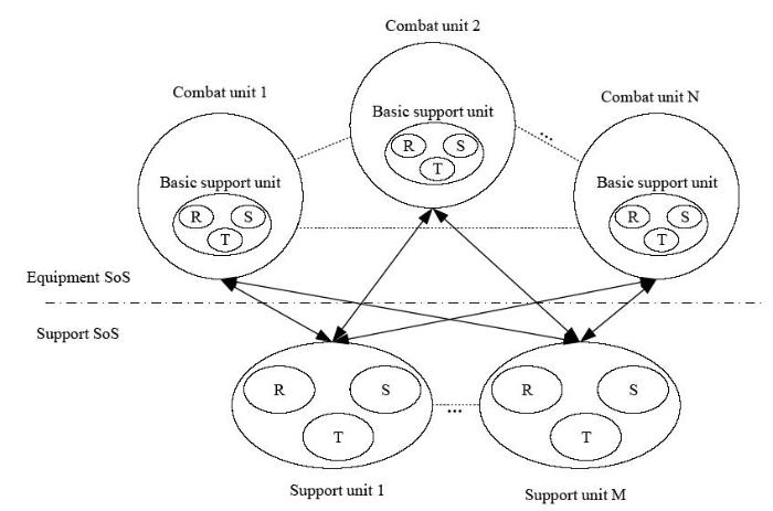
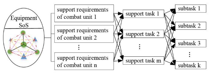
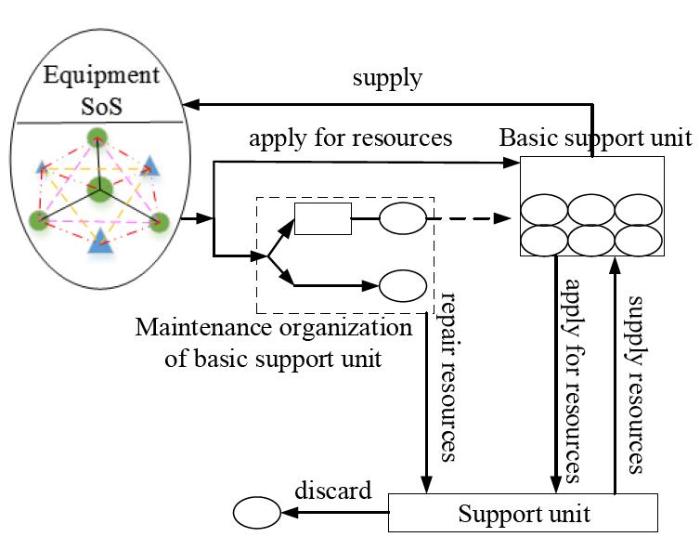
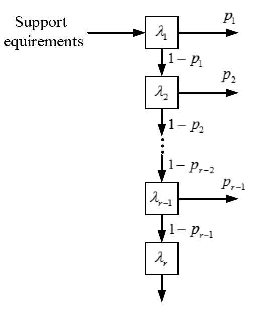
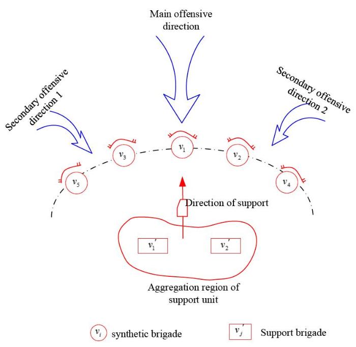
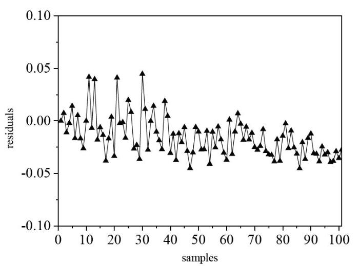

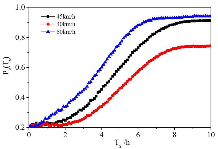
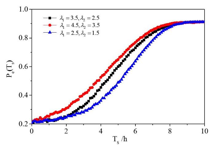
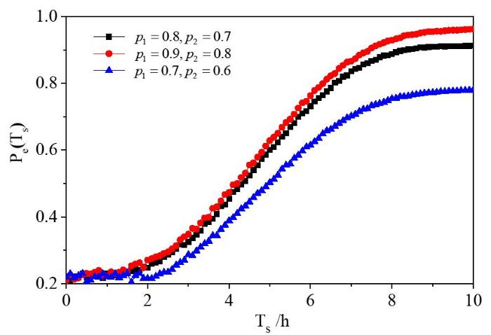
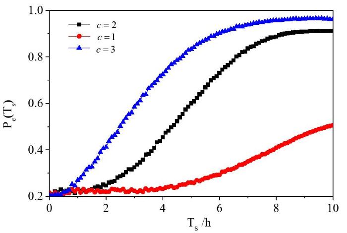
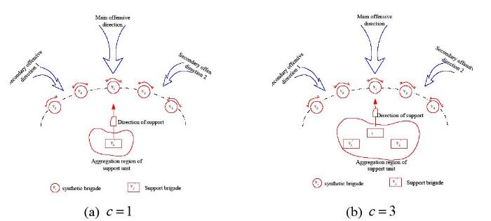

