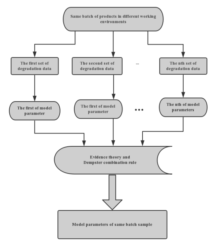
The degradation analysis of products has been demonstrated as a significant toolkit for reliability analysis. Data from the same batch of products in different working environments cannot be directly used to analyze product reliability. In this paper, motivated by this circumstance, we first assume that degradation data sets from different working environments are subject to different inverse Gaussian process models, and maximum likelihood estimation is used to obtain multiple model parameters. Secondly, we construct evidence by quantifying different information of products, apply the evidence theory to fuse model parameters, and then analyze the reliability of products from the same batch. Finally, we use performance degradation data of the laser to illustrate the method.
Yuwei Wang, Hailin Feng. Reliability Analysis based on Inverse Gauss Degradation Process and Evidence Theory. International Journal of Performability Engineering, 2019, 15(2): 353-361 doi:10.23940/ijpe.19.02.p1.353361
Performance degradation is the evolution process of the state during the failure process. It is different from traditional failure-based product life information data. Performance degradation data mainly concerns the failure process information related to product life. Through the analysis and study of the failure mechanism of the product, the related performance characteristics that can reflect the life or reliability of the product are selected. The characteristic variables are called performance degradation, and the failure process of the product is described quantitatively. Compared with the traditional product information based on failure life, performance-based degradation products include more product implicit information, making up for the effect of failure data to ignore the initial performance difference between products. With the fast development of the defense industry and advanced manufacturing technology, the failure data of products is difficult to collect.
With the development of monitoring technology, more and more performance degradation information can be collected in the working state of the product. Based on performance degradation data, modeling and analysis product reliability has become significant. Performance degradation is a highly correlated physical variable with product life. We usually describe the variation laws of the degradation path of products with time asa stochastic process. In order to reduce the number of parameters of theWiener degradation process while considering the relationship between individual variance and population variance, life data and degradation data were fused to analyze the reliability of the blowout preventer valve [1]. Unlike the Wiener degradation process, the gamma degradation process describes a monotonic degradation process thatmakes up for the discontinuity of the Wiener process[2]. However, engineering practice shows that some degenerate data cannot be simply described by the Wiener or gamma process. The IGprocess also has independent incremental properties. Some scholars have introduced it into the modeling of product performance degradation. The IGprocess is an independent but not necessarily identically distributed gamma process in the extreme case [3]. It can be used to analyze remaining useful life and product reliability [4-7]. The stochastic degradation process model was used to analyze the reliability of the product, and the key problem was to obtain more accurate model parameters with the data collected. The concept of degenerated mean function was proposed, three different degradation rates were discussed, and the IG degradation process model parameters were estimated by the Bayesian theory [8]. The IG process was used to model the degradation data of oil and gas pipelines corrosion, andthe empirical maximization algorithm and particle filter algorithm were combined to estimate the parameters of the model [9]. A competitive failure model was constructed with the IG degradation process, and MLE was used to evaluate the model parameters [5]. Based on the inverse Gaussian process, a two-stage Bayesian method was introduced to implement parameter estimation [10]. It is note worthy that all the analysis methods listed above have been studied under the same means of data collection, from the same or similar work environment. In order to analyze the product status under different environments and fuse multi-source information, the evidence theory was proposed and applied to reliability data processing. Evidence theory is a complete theory dealing with uncertainty. It can emphasize not only the objectivity of things, but also the subjectivity of human’s estimation of things[11-13]. The prior data required by the evidence theory is more intuitive and easier to obtain than that in the probabilistic inference theory, and the description of uncertain problems is flexible. By synthesizing the knowledge and data of different experts or data sources, the description of uncertain problems is more flexible and convenient. The concept of attribute weight was proposed, and ER was used to fuse the model parameters[14]. The angle cosine similarity coefficient and its similarity matrix were used as the weight of the data to improve the D-S evidence theory and analyze the reliability of a diesel engine [15].
We have noticed little research on discrepant datain different working environments. If the discrepant data has been forcibly used to estimate model parameters, the results of the analysis will be inaccurate. In practical engineering, especially for complex products or systems, reliability analyses under different working environments will contain various kinds of uncertainty, and common analysis methods are not perfect for multi-source information processing in different environments. The evidence theory has certain advantages in dealing with probabilistic uncertainty, and it can effectively fuse multi-source uncertain information in different environments. However, it is still a challenge to evaluate the reliability of performance degradation products with discrepant data under different environments.
The outline of this paper is as follows. In Section 2, the IG degradation process is introduced into data modeling, and MLE is adopted to estimate the model parameters. In Section 3, the model parameters are fused with the combined evidence theory and the information of different products in the same batch. In Section 4, the idea of the algorithmis summarized. In Section 5, the method is examined by a numerical example involving a laser. In Section 6, conclusions for performance degradation product reliability analysis based on evidence theory are presented.
2. Inverse Gauss Process and Evidence Theory Degenerate Modeling Method
The following will be divided into two parts to discuss. The first parte stablishes the IG process model and estimation parameter, and the other part elaborates on the model parameter fusion algorithm based on the evidence theory.
2.1. The Model of the IG Process
For a batch of performance degradation products, only a small amount of degradation data can be obtained due to technical and budgetary constraints. Suppose the degradation data set of the product is $\left\{ \left( {{t}_{i}}, {{y}_{i}} \right)i=1, 2, \cdots, n \right\}$${{t}_{i}}\in R, $ and the ith monitoring time ${{y}_{i}}\in R, $ is the product degradation at the corresponding time. The product degradation path $\left\{ Y(t), t\ge 0 \right\}$ obeys the inverse Gaussian process degradation model and hasthe following properties [16]:
·$Y(t)\equiv 0$.
·For any ${{t}_{2}}>{{t}_{1}}\ge {{s}_{2}}>{{s}_{1}}$, $Y({{t}_{2}})-Y({{t}_{1}})$ and $Y({{s}_{2}})-Y({{s}_{1}})$ are independent degenerate increments.
Parametric $\Lambda (t)$ is a function of monotonous growth that has a clear physical meaning and describes the mean of the degenerate process. We can use $\Lambda (t)$ to define the different product degradation rate $r(t). $When the degradation rate $r(t)$ is the linear and the monotonic function separately, the corresponding degradation mean functions are obtained [8]:
Where $\beta$ and $\eta$ are the shape parameter and scale parameter respectively, and $\mu $ is a constant. We havethe probability density function of $y(t)$:
When the product performance degradation reaches the preset failure threshold, $T=\left\{ \left. t \right|y(t)\ge D \right\}$, and we define this as product failure. Considering the monotony of the IG process, the reliability function of the product is defined as [3]:
We have product degradation data $\left\{ y({{t}_{1}}), y({{t}_{2}}), y({{t}_{3}}), \cdots, y({{t}_{n}}) \right\}$, and the products havean independent degenerate increment $\Delta Y=\left\{ \Delta {{y}_{1}}, \Delta {{y}_{2}}, \cdots, \Delta {{y}_{n}} \right\}$.
$y(0)\equiv 0$, and $\Delta y=y(t+\Delta t)-y(t)\tilde{\ }IG(\Delta \Lambda, \lambda \Delta {{\Lambda }^{2}})$ obeys an IG distribution.
We use MLE to calculate IG degenerate model parameters. When the product degenerate increment $\Delta {{y}_{i}}\text{ }\!\!\tilde{\ }\!\!\text{ }IG $$(\Delta \Lambda, \lambda \Delta {{\Lambda }^{2}}), \text{ }i=1, \cdots, n, \text{ }\Delta \Lambda >0, \text{ }\lambda >0$, obtain the likelihood function of parameters ${{\theta }_{IG}}=(\Lambda (t), \lambda )$:
Let $L({{\theta }_{IG}})$ have a partial derivative of 0 on $\Delta \Lambda (t), \text{ }\lambda $, and then the MLE of the IG model parameter $L({{\theta }_{IG}})$is:
If the different product degradation data does not have the discrepancy or the discrepant data can be ignored, the data can be used directly to estimate the parameters $\Lambda \Delta (t)$ and $\lambda $.
For the discrepant data of the same batch of products, different degenerate data should have different degrees of importance in the estimation of the parameter for thedegeneration model.
3. Multi-Source Information Fusion based on Evidence Theory
Evidence theory has a certain advantage in dealing with multiple source uncertain information: it satisfies a weaker condition than the Bayesian probability theory. It can emphasize the objectivity of things and the subjectivity of human’s estimation of things.
Theset of possible even information in different environments is defined as the frame of discernment. It is also the assumed space for information that all even may imply, denoted as $\Theta $. A subset of the frame of discernment is called a proposition. Evidence is designed by experts based on propositions. Define the basic probability assignment to describe the trust degree based on the frame of discernment, represented as a probability that possible events given in a function, usually recorded as the $m$ function, reflect the reliability of A. The following conditions must be satisfied [17]:
${{2}^{\Theta }}$ is a power set of the frame of discernment$\Theta $, anda power set is a collection of subsets of a set.
The discrepant degenerate data are subject to different IG degradation process models, and the multiple degenerate data has multiple model parameters. Let each model parameterbe an element of the frame of discernment $\Theta =\left\{ {{\alpha }_{1}}, {{\alpha }_{2}}, \cdots, {{\alpha }_{n}} \right\}$. BPA describes the trust degree to discrepant data under the different evidence. Determine the probability of the estimated parameters in each working environment for different evidence. Obtain the model parameters for products in different working environments, the volume of the sample data, and the parameter deviation degree. The rules of definition are as follows.
3.1. Data Sample Capacity
Under the frame of discernment, the BPA function of the sample size of the product data in different environments can be obtained by calculating the percentage of the sample size directly. However, this can easily cause small sample information to be diluted and even ignored in the fusion. We calculate the logarithm of the sample size and the corresponding percentage and then obtain the BPA function under the evidence of product data sample capacity [16].
Suppose there are $n$ groups of sample degenerate data, $Y=\left\{ {{y}_{1}}, {{y}_{2}}, \cdots, {{y}_{n}} \right\}, \text{ }{{y}_{i}}=\left\{ {{\partial }_{i1}}, {{\partial }_{i2}}, \cdots, {{\partial }_{ij}} \right\}, \text{ (}i=1, 2\cdots, n), \text{ }i$ is the number of sample degenerate data in different environment experimental products, $j$ is the number of discrete points in the degraded monitoring time, and ${{\partial }_{ij}}$ is the product degradation in the monitoring time $j$. For the parameters estimated in the degenerate data of group $i$, the BPA function under the evidence of data sample size is as follows:
To avoid biased estimates of the parameters and large deviations of the product path and overall degeneracy path, the corresponding data should be assigned a small weight.
For multiple model parameters ${{\alpha }_{1}}, {{\alpha }_{2}}, \cdots, {{\alpha }_{n}}$, we get the mean value $\alpha =\frac{1}{n}\sum\nolimits_{i=1}^{n}{{{\alpha }_{i}}}.$
Calculate the deviation of each parameter from the mean value; the greaterthe deviation from the total mean value, the higher the uncertainty and the lower the level of importance. Therefore, according to the reciprocal of distance as a criterion, define the BPA function under the evidence of the parameter deviation degree as
According to the authority of experts, the importance of each product in the same batch of products is given. The closer the data work environment is to the current environment, the higher the weight that should be given. The BPA function defined by expertise evidence is
In solving practical problems, experts design various evidence, calculate every evidence of power set elements of trust, trust all the evidence, and then calculate the comprehensive trust of all evidence of events.
For ${{A}_{i}}\subseteq \Theta $under the frame of discernment, there is a finite number of BPA ${{m}_{1}}, {{m}_{2}}, \cdots, {{m}_{n}}, $ and Dempster’s combination rule is shown below:
The brightness of the laser will gradually decrease with an increase in the use time. To keep the laser brightness at a constant working level, we need to increase the working current over time. Define product failure when the operating current increases to a fixed threshold. The laser data used in this paper was obtained in different environments with different sample sizes. We use this data as an example to prove the validity and feasibility of the proposed method.
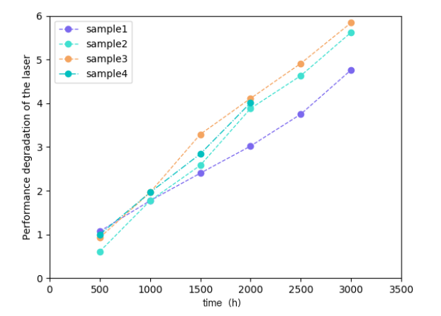
A performance indicator increases the percentage of the operating current. The degradation data of four test products are measured in this paper. In addition to one product, the other three products were monitored at six equal interval dispersion points. The following Table 1 and Figure 2show the degradation test data and the corresponding degradation path.
Figure 2.
Performance degradation trajectory of laser
An IG process model is used to fit the degenerated data of the laser, and it is shown that the degradation process conforms to the IG process [2]. According to expert experience, the process of laser degradation obeys a linear path. Therefore, establishing an IG degradation process mode $IG(\Lambda (t), \lambda \Lambda {{(t)}^{2}})$, $\Lambda (t)=\mu t, \text{ }u>0$ is a constant degradation rate.Using the MLE method to obtain the parameter ${{\Theta }_{IG}}=\left( \Lambda (t), \lambda \right)$ in the model, obtain four sets of parameter values, shown in Table 2.
Under the framework of evidence reasoning, the method proposed in this paperis used. Based on the product degradation test data and the BPA of different evidences, the sample size, deviation informationof parameter mean value, and expertise are calculated. Dempster’s combination rule is applied to get the proportion of importance of each product model parameter after the fusion of multi-source evidence, the fused parameter $\Lambda (t)$ and $\lambda$ are shown in Table 3 and Table 4respectively.
The method of weighted averages is utilized to obtain the parameters of the IG process model as $\Lambda (t)=0.9325t, \text{ }\lambda =0.0376$.
According to engineering experience, the operating current of the laser is increased by 10% from the initial current. We judge the failure of the product. Substituting the failure threshold $(D=10)$ and the corresponding model parameters $\Lambda (t)=0.9325t, \text{ }\lambda =0.0376$ into (4), the analytical expression of the laser reliability under multi-source information is obtained:
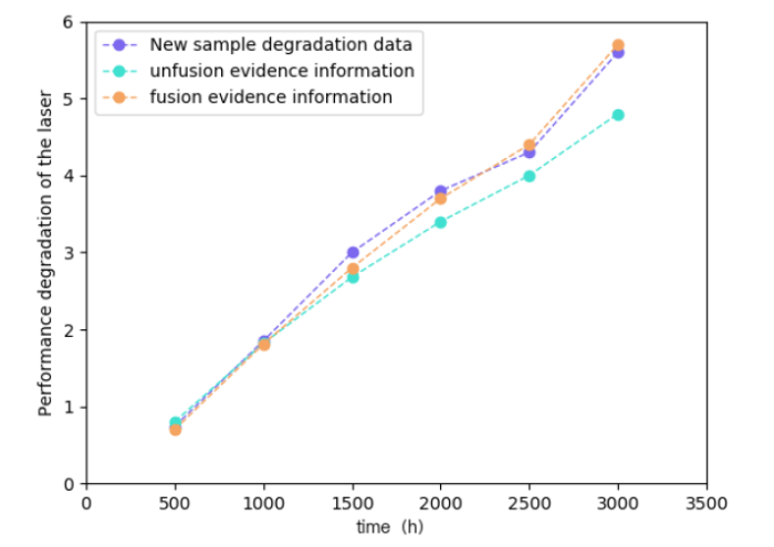
In order to further prove the validity and practicality of the proposed method, the same four sets oflaser degradation data are used, but the sample data of these products are directly combined into one sample set. The parameters of the corresponding model are obtained as respectively. Use OpenBUGS software and Monte Carlo simulations to obtain the model parameters under the above two methods. Assume that the parameters are unconditionally a priori and each group produces 5000 degenerate data, and then calculate the average degradation value of the product. Finally, compare the results with a set of product performance degradation data collected in real-time, simulation comparison results and corresponding trajectories are shown in Table 5 and Figure 3.
Table 5
Table 5.Fusion and infusion information degradation prediction comparison
Figure 3.
Fusion and infusion information degradation prediction comparison
It can be seen that the infused degradation samples obtained using the simulation are affected by the first set of deviation samples, and this causes the macro forecast value to be relatively low. Through expert experience, we know that sample3 is closest to the new sample working environment. Therefore, sample3 should receive more attention. After assigning the weight, the fusion sample obtained from the simulation is closest to the new real sample. To some extent, the impact of discrepancies in product sample data is avoided.
6. Conclusions
To address discrepancies in degradation data of the same batch of products, a degenerate modeling method combining evidence theory and IG process is proposed. After the fusion of data, the degradation model can be established more accurately, making up for the problem of inaccurate product reliability analysis caused by the simple combination of data. Bydisplaying and analyzing the degenerate data of a laser, fusionof differentinformation from the same batch product data to achieve accurate analysis product reliability index provides a novel idea.
61The system07s deterioration is modeled by a non-homogeneous gamma process.61The observations are noisy with an additive Gaussian noise.61The system Remaining Useful Lifetime (RUL) is estimated through MCMC methods.61RUL based maintenance policies are proposed.
Z.S.Ye and N. Chen,
“The Inverse Gaussian Process as a Degradation Model, ”
Proceedings of Technometrics, Vol. 56, No. 3, pp.302-311, 2014
This article systematically investigates the inverse Gaussian (IG) process as an effective degradation model. The IG process is shown to be a limiting compound Poisson process, which gives it a meaningful physical interpretation for modeling degradation of products deteriorating in random environments. Treated as the first passage process of a Wiener process, the IG process is flexible in incorporating random effects and explanatory variables that account for heterogeneities commonly observed in degradation problems. This flexibility makes the class of IG process models much more attractive compared with the Gamma process, which has been thoroughly investigated in the literature of degradation modeling. The article also discusses statistical inference for three random effects models and model selection. It concludes with a real world example to demonstrate the applicability of the IG process in degradation analysis. Supplementary materials for this article are available online.
F. DuanandG.Wang,
“Reliability Modeling of Two-Phase Inverse Gaussian Degradation Process, ”
in Proceedings of the Second International Conference on Reliability Systems Engineering, IEEE, pp.1-6, 2017
This paper discusses the reliability evaluation of the two-phase model with the inverse Gaussian (IG) process. In the two phases, the degradation paths are supposed to follow the IG process with different parameters. To represent the subject-to-subject heterogeneity, the change points and the model parameters of different devices are set to be different. For each device, the change point is detected based on the Schwarz information criterion (SIC), and the unknown parameters are obtained by utilizing the maximum likelihood estimation (MLE) approach. Furthermore, the reliability function of each device under the discussed two-phase IG model is also computed. Finally, an example of liquid coupling devices (LCDs) is presented to validate the proposed model, and it can be found that the proposed model fits this data set well.
H.Guo, T.Zhang, L. Y.Ping, E. S.Pan,
“Research on Competing Failure Modeling based on the Inverse Gaussian Process, ”
in Proceedings of Industrial Engineering and Management, Vol. 22, No. 1, pp. 89-94, 2017
The use of degradation data to estimate the remaining useful life (RUL) has gained great attention with the widespread use of prognostics and health management on safety critical systems. Accurate RUL estimation can prevent system failure and reduce the running risks since the efficient maintenance service could be scheduled in advance. In this paper, we present a degradation modeling and RUL estimation approach by using available degradation data for a deteriorating system. An inverse Gaussian process with the random effect is firstly used to characterize the degradation process of the system. Expectation maximization algorithm is then adopted to estimate the model parameters, and the random parameters in the degradation model are updated by Bayesian method, which makes the estimated RUL able to be real-time updated in terms of the fresh degradation data. Our proposed method can capture the latest condition of the system by means of updating degradation data continuously, and obtain the explicit expression of RUL distribution. Finally, a numerical example and a practical case study are provided to show that the presented approach can effectively model degradation process for the individual system and obtain better results for RUL estimation.
Y.Zhou, L.V. Wei-Min, and Y.Sun,
“Fusion Prediction Method for the Life of MEMS Accelerometer based on Inverse Gaussian Process, ”
Degradation observations of modern engineering systems, such as manufacturing systems, turbine engines, and high-speed trains, often demonstrate various patterns of time-varying degradation rates. General degradation process models are mainly introduced for constant degradation rates, which cannot be used for time-varying situations. Moreover, the issue of sparse degradation observations and the problem of evolving degradation observations both are practical challenges for the degradation analysis of modern engineering systems. In this paper, parametric inverse Gaussian process models are proposed to model degradation processes with constant, monotonic, and S-shaped degradation rates, where physical meaning of model parameters for time-varying degradation rates is highlighted. Random effects are incorporated into the degradation process models to model the unit-to-unit variability within product population. A general Bayesian framework is extended to deal with the degradation analysis of sparse degradation observations and evolving observations. An illustrative example derived from the reliability analysis of a heavy-duty machine tool's spindle system is presented, which is characterized as the degradation analysis of sparse degradation observations and evolving observations under time-varying degradation rates.
X.Zhang, Y.Li, X.Wang,
“Maintenance Strategy of Corroded Oil-Gas Pipeline based on Inverse Gaussian Process, ”
in Proceedings of Acta Petrolei Sinica, Vol. 38, No. 3, pp.356-362, 2017
Modern engineering systems are generally composed of multicomponents and are characterized as multifunctional. Condition monitoring and health management of these systems often confronts the difficulty of degradation analysis with multiple performance characteristics. Degradation observations generally exhibit an s-dependent nature and sometimes experience incomplete measurements. These issues necessitate investigating multiple s-dependent degradations analysis with incomplete observations. In this paper, a new type of bivariate degradation model based on inverse Gaussian processes and copulas is proposed. A two-stage Bayesian method is introduced to implement parameter estimation for the bivariate degradation model by treating the degradation processes and copula function separately. Degradation inferences for missing observation points, and for future observation points are investigated. A simulation study is presented to study the effectiveness of the dependence modeling and degradation inference of the proposed method. For demonstration, a bivariate degradation analysis of positioning accuracy and output power of heavy machine tools subject to incomplete measurements is provided.
F.Ye, J.Chen, andY.Li,
“Improvement of D-S Evidence Theory for Multi-Sensor Conflicting Information, ”
ABSTRACT A new evidential reasoning based approach is proposed that may be used to deal with uncertain decision knowledge in multiple-attribute decision making (MADM) problems with both quantitative and qualitative attributes. This approach is based on an evaluation analysis model and the evidence combination rule of the Dempster-Shafer theory. It is akin to a preference modeling approach, comprising an evidential reasoning framework for evaluation and quantification of qualitative attributes. Two operational algorithms have been developed within this approach for combining multiple uncertain subjective judgments. Based on this approach and a traditional MADM method, a decision making procedure is proposed to rank alternatives in MADM problems with uncertainty. A numerical example is discussed to demonstrate the implementation of the proposed approach. A multiple-attribute motor cycle evaluation problem is then presented to illustrate the hybrid decision making procedure
Z.Zhang, C.Jiang, X. X.Ruan, and F. J.Guan,
“A Novel Evidence Theory Model Dealing with Correlated Variables and the Corresponding Structural Reliability Analysis Method, ”
Evidence theory serves as a powerful tool to deal with epistemic uncertainty which widely exists in the design stages of many complex engineering systems or products. However, the traditional evidence
L. F.Ming, C. H.Hu, Z. J.Zhou, P.Wang,
“A degradation Modeling Method based on Inverse Gaussian Process and Evidential Reasoning, ”
in Proceedings of Electronics Optics & Control, Vol. 22, No. 1, pp. 92-96, 2015
The problem of residual life prediction of high-reliability device was studied. Considering the lack of life data and the difficulty in establishing a physical model, we used the inverse Gaussian regression model to build up the degradation process model of device in combination with the monotonous degradation data.Then we obtained the degradation model by using the method of parameter estimation for forecasting the residual life of device. The problem of data fusion may emerge when there are data of multiple sets in the same batch to estimate inverse Gaussian model parameter. We used the method based on Evidential Reasoning( ER) to fuse the multi-source data, and put forward the concept of attribute weights, in order to estimate the inverse Gaussian model parameters more accurately. Finally, simulation experiment, proved that the presented method can obtain more reliable parameter estimation results.
L.Liang, Y.Shen, Q .Cai, and Y.Gu,
“A Reliability Data Fusion Method based on Improved D-S Evidence Theory, ”
in Proceedings of International Conference on Reliability, Maintainability and Safety, IEEE, pp.1-6, 2017
In order to solve the problem of the uncertainty of multi-source reliability data, a reliability data fusion method based on improved D-S evidence theory was presented. The confidence level was calculated by using the angle cosine similarity coefficient and its similarity matrix which is as the weight of the data. After the weights are assigned again, they are fused together with the information. By using this method, the causes of the faults can be determined. A major problem that the fusion results are inconsistent with the intuition when the multi-source data information conflicts each other was solved. A case of reliability analysis of a certain diesel engine was presented as an example to illustrate the proposed method. The results showed that the interference of conflicting evidence can be reduced by introducing a similarity coefficient. Furthermore, the fusion efficiency and precision of the model are increased. Not only can the real reasons for the diesel engine faults be identified accurately, but also the identification efficiency of the whole system can be improved.
H.Wang, G. J.Wang, F. J.Duan,
“Planning of Step-Stress Accelerated Degradation Test based on the Inverse Gaussian Process, ”
Reliability Engineering & System Safety, Vol. 154, pp.97-105, 2016
The paper proposes a parallel survey of revision and updating operations available in the probability theory and in the possibility theory frameworks. In these two formalisms the current state of knowledge is generally represented by a [0, 1]-valued function whose domain is an exhaustive set of mutually exclusive possible states of the world. However, in possibility theory, the unit-interval can be viewed as a purely ordinal scale. Two general kinds of operations can be defined on this assignment function: conditioning, and imaging (projection). Counterparts to these operations are presented for the possibilistic framework including the case of conditioning upon uncertain observations, and justifications are given which parallel the ones existing for the probabilistic operations. More particularly, it is recalled that possibilistic conditioning satisfies all the postulates proposed by (Alchourron et al., 1985) for belief revision (stated in possibilistic terms), and it is proved that possibilistic imaging satisfies all the postulates proposed by Katsuno and Mendelzon (1991)
“Remaining Lifetime Prediction of Blowout Preventer Valve based on Fusion of Lifetime Data and Degradation Data, ”
1
2017
... With the development of monitoring technology, more and more performance degradation information can be collected in the working state of the product. Based on performance degradation data, modeling and analysis product reliability has become significant. Performance degradation is a highly correlated physical variable with product life. We usually describe the variation laws of the degradation path of products with time asa stochastic process. In order to reduce the number of parameters of theWiener degradation process while considering the relationship between individual variance and population variance, life data and degradation data were fused to analyze the reliability of the blowout preventer valve [1]. Unlike the Wiener degradation process, the gamma degradation process describes a monotonic degradation process thatmakes up for the discontinuity of the Wiener process[2]. However, engineering practice shows that some degenerate data cannot be simply described by the Wiener or gamma process. The IGprocess also has independent incremental properties.Some scholars have introduced it into the modeling of product performance degradation. The IGprocess is an independent but not necessarily identically distributed gamma process in the extreme case [3]. It can be used to analyze remaining useful life and product reliability [4-7]. The stochastic degradation process model was used to analyze the reliability of the product, and the key problem was to obtain more accurate model parameters with the data collected. The concept of degenerated mean function was proposed, three different degradation rates were discussed, and the IG degradation process model parameters were estimated by the Bayesian theory [8]. The IG process was used to model the degradation data of oil and gas pipelines corrosion, andthe empirical maximization algorithm and particle filter algorithm were combined to estimate the parameters of the model [9]. A competitive failure model was constructed with the IG degradation process, and MLE was used to evaluate the model parameters [5]. Based on the inverse Gaussian process, a two-stage Bayesian method was introduced to implement parameter estimation [10]. It is note worthy that all the analysis methods listed above have been studied under the same means of data collection, from the same or similar work environment.In order to analyze the product status under different environments and fuse multi-source information, the evidence theory was proposed and applied to reliability data processing. Evidence theory is a complete theory dealing with uncertainty.It can emphasize not only the objectivity of things, but also the subjectivity of human’s estimation of things[11-13]. The prior data required by the evidence theory is more intuitive and easier to obtain than that in the probabilistic inference theory, and the description of uncertain problems is flexible. By synthesizing the knowledge and data of different experts or data sources, the description of uncertain problems is more flexible and convenient. The concept of attribute weight was proposed, and ER was used to fuse the model parameters[14]. The angle cosine similarity coefficient and its similarity matrix were used as the weight of the data to improve the D-S evidence theory and analyze the reliability of a diesel engine [15]. ...
“Remaining Useful Lifetime Estimation and Noisy Gamma Deterioration Process, ”
2
2016
... With the development of monitoring technology, more and more performance degradation information can be collected in the working state of the product. Based on performance degradation data, modeling and analysis product reliability has become significant. Performance degradation is a highly correlated physical variable with product life. We usually describe the variation laws of the degradation path of products with time asa stochastic process. In order to reduce the number of parameters of theWiener degradation process while considering the relationship between individual variance and population variance, life data and degradation data were fused to analyze the reliability of the blowout preventer valve [1]. Unlike the Wiener degradation process, the gamma degradation process describes a monotonic degradation process thatmakes up for the discontinuity of the Wiener process[2]. However, engineering practice shows that some degenerate data cannot be simply described by the Wiener or gamma process. The IGprocess also has independent incremental properties.Some scholars have introduced it into the modeling of product performance degradation. The IGprocess is an independent but not necessarily identically distributed gamma process in the extreme case [3]. It can be used to analyze remaining useful life and product reliability [4-7]. The stochastic degradation process model was used to analyze the reliability of the product, and the key problem was to obtain more accurate model parameters with the data collected. The concept of degenerated mean function was proposed, three different degradation rates were discussed, and the IG degradation process model parameters were estimated by the Bayesian theory [8]. The IG process was used to model the degradation data of oil and gas pipelines corrosion, andthe empirical maximization algorithm and particle filter algorithm were combined to estimate the parameters of the model [9]. A competitive failure model was constructed with the IG degradation process, and MLE was used to evaluate the model parameters [5]. Based on the inverse Gaussian process, a two-stage Bayesian method was introduced to implement parameter estimation [10]. It is note worthy that all the analysis methods listed above have been studied under the same means of data collection, from the same or similar work environment.In order to analyze the product status under different environments and fuse multi-source information, the evidence theory was proposed and applied to reliability data processing. Evidence theory is a complete theory dealing with uncertainty.It can emphasize not only the objectivity of things, but also the subjectivity of human’s estimation of things[11-13]. The prior data required by the evidence theory is more intuitive and easier to obtain than that in the probabilistic inference theory, and the description of uncertain problems is flexible. By synthesizing the knowledge and data of different experts or data sources, the description of uncertain problems is more flexible and convenient. The concept of attribute weight was proposed, and ER was used to fuse the model parameters[14]. The angle cosine similarity coefficient and its similarity matrix were used as the weight of the data to improve the D-S evidence theory and analyze the reliability of a diesel engine [15]. ...
... An IG process model is used to fit the degenerated data of the laser, and it is shown that the degradation process conforms to the IG process [2].According to expert experience, the process of laser degradation obeys a linear path. Therefore, establishing an IG degradation process mode $IG(\Lambda (t), \lambda \Lambda {{(t)}^{2}})$, $\Lambda (t)=\mu t, \text{ }u>0$ is a constant degradation rate.Using the MLE method to obtain the parameter ${{\Theta }_{IG}}=\left( \Lambda (t), \lambda \right)$ in the model, obtain four sets of parameter values, shown in Table 2. ...
“The Inverse Gaussian Process as a Degradation Model, ”
2
2014
... With the development of monitoring technology, more and more performance degradation information can be collected in the working state of the product. Based on performance degradation data, modeling and analysis product reliability has become significant. Performance degradation is a highly correlated physical variable with product life. We usually describe the variation laws of the degradation path of products with time asa stochastic process. In order to reduce the number of parameters of theWiener degradation process while considering the relationship between individual variance and population variance, life data and degradation data were fused to analyze the reliability of the blowout preventer valve [1]. Unlike the Wiener degradation process, the gamma degradation process describes a monotonic degradation process thatmakes up for the discontinuity of the Wiener process[2]. However, engineering practice shows that some degenerate data cannot be simply described by the Wiener or gamma process. The IGprocess also has independent incremental properties.Some scholars have introduced it into the modeling of product performance degradation. The IGprocess is an independent but not necessarily identically distributed gamma process in the extreme case [3]. It can be used to analyze remaining useful life and product reliability [4-7]. The stochastic degradation process model was used to analyze the reliability of the product, and the key problem was to obtain more accurate model parameters with the data collected. The concept of degenerated mean function was proposed, three different degradation rates were discussed, and the IG degradation process model parameters were estimated by the Bayesian theory [8]. The IG process was used to model the degradation data of oil and gas pipelines corrosion, andthe empirical maximization algorithm and particle filter algorithm were combined to estimate the parameters of the model [9]. A competitive failure model was constructed with the IG degradation process, and MLE was used to evaluate the model parameters [5]. Based on the inverse Gaussian process, a two-stage Bayesian method was introduced to implement parameter estimation [10]. It is note worthy that all the analysis methods listed above have been studied under the same means of data collection, from the same or similar work environment.In order to analyze the product status under different environments and fuse multi-source information, the evidence theory was proposed and applied to reliability data processing. Evidence theory is a complete theory dealing with uncertainty.It can emphasize not only the objectivity of things, but also the subjectivity of human’s estimation of things[11-13]. The prior data required by the evidence theory is more intuitive and easier to obtain than that in the probabilistic inference theory, and the description of uncertain problems is flexible. By synthesizing the knowledge and data of different experts or data sources, the description of uncertain problems is more flexible and convenient. The concept of attribute weight was proposed, and ER was used to fuse the model parameters[14]. The angle cosine similarity coefficient and its similarity matrix were used as the weight of the data to improve the D-S evidence theory and analyze the reliability of a diesel engine [15]. ...
... When the product performance degradation reaches the preset failure threshold, $T=\left\{ \left. t \right|y(t)\ge D \right\}$, and we define this as product failure. Considering the monotony of the IG process, the reliability function of the product is defined as [3]: ...
“Reliability Modeling of Two-Phase Inverse Gaussian Degradation Process, ”
1
2017
... With the development of monitoring technology, more and more performance degradation information can be collected in the working state of the product. Based on performance degradation data, modeling and analysis product reliability has become significant. Performance degradation is a highly correlated physical variable with product life. We usually describe the variation laws of the degradation path of products with time asa stochastic process. In order to reduce the number of parameters of theWiener degradation process while considering the relationship between individual variance and population variance, life data and degradation data were fused to analyze the reliability of the blowout preventer valve [1]. Unlike the Wiener degradation process, the gamma degradation process describes a monotonic degradation process thatmakes up for the discontinuity of the Wiener process[2]. However, engineering practice shows that some degenerate data cannot be simply described by the Wiener or gamma process. The IGprocess also has independent incremental properties.Some scholars have introduced it into the modeling of product performance degradation. The IGprocess is an independent but not necessarily identically distributed gamma process in the extreme case [3]. It can be used to analyze remaining useful life and product reliability [4-7]. The stochastic degradation process model was used to analyze the reliability of the product, and the key problem was to obtain more accurate model parameters with the data collected. The concept of degenerated mean function was proposed, three different degradation rates were discussed, and the IG degradation process model parameters were estimated by the Bayesian theory [8]. The IG process was used to model the degradation data of oil and gas pipelines corrosion, andthe empirical maximization algorithm and particle filter algorithm were combined to estimate the parameters of the model [9]. A competitive failure model was constructed with the IG degradation process, and MLE was used to evaluate the model parameters [5]. Based on the inverse Gaussian process, a two-stage Bayesian method was introduced to implement parameter estimation [10]. It is note worthy that all the analysis methods listed above have been studied under the same means of data collection, from the same or similar work environment.In order to analyze the product status under different environments and fuse multi-source information, the evidence theory was proposed and applied to reliability data processing. Evidence theory is a complete theory dealing with uncertainty.It can emphasize not only the objectivity of things, but also the subjectivity of human’s estimation of things[11-13]. The prior data required by the evidence theory is more intuitive and easier to obtain than that in the probabilistic inference theory, and the description of uncertain problems is flexible. By synthesizing the knowledge and data of different experts or data sources, the description of uncertain problems is more flexible and convenient. The concept of attribute weight was proposed, and ER was used to fuse the model parameters[14]. The angle cosine similarity coefficient and its similarity matrix were used as the weight of the data to improve the D-S evidence theory and analyze the reliability of a diesel engine [15]. ...
“Research on Competing Failure Modeling based on the Inverse Gaussian Process, ”
1
2017
... With the development of monitoring technology, more and more performance degradation information can be collected in the working state of the product. Based on performance degradation data, modeling and analysis product reliability has become significant. Performance degradation is a highly correlated physical variable with product life. We usually describe the variation laws of the degradation path of products with time asa stochastic process. In order to reduce the number of parameters of theWiener degradation process while considering the relationship between individual variance and population variance, life data and degradation data were fused to analyze the reliability of the blowout preventer valve [1]. Unlike the Wiener degradation process, the gamma degradation process describes a monotonic degradation process thatmakes up for the discontinuity of the Wiener process[2]. However, engineering practice shows that some degenerate data cannot be simply described by the Wiener or gamma process. The IGprocess also has independent incremental properties.Some scholars have introduced it into the modeling of product performance degradation. The IGprocess is an independent but not necessarily identically distributed gamma process in the extreme case [3]. It can be used to analyze remaining useful life and product reliability [4-7]. The stochastic degradation process model was used to analyze the reliability of the product, and the key problem was to obtain more accurate model parameters with the data collected. The concept of degenerated mean function was proposed, three different degradation rates were discussed, and the IG degradation process model parameters were estimated by the Bayesian theory [8]. The IG process was used to model the degradation data of oil and gas pipelines corrosion, andthe empirical maximization algorithm and particle filter algorithm were combined to estimate the parameters of the model [9]. A competitive failure model was constructed with the IG degradation process, and MLE was used to evaluate the model parameters [5]. Based on the inverse Gaussian process, a two-stage Bayesian method was introduced to implement parameter estimation [10]. It is note worthy that all the analysis methods listed above have been studied under the same means of data collection, from the same or similar work environment.In order to analyze the product status under different environments and fuse multi-source information, the evidence theory was proposed and applied to reliability data processing. Evidence theory is a complete theory dealing with uncertainty.It can emphasize not only the objectivity of things, but also the subjectivity of human’s estimation of things[11-13]. The prior data required by the evidence theory is more intuitive and easier to obtain than that in the probabilistic inference theory, and the description of uncertain problems is flexible. By synthesizing the knowledge and data of different experts or data sources, the description of uncertain problems is more flexible and convenient. The concept of attribute weight was proposed, and ER was used to fuse the model parameters[14]. The angle cosine similarity coefficient and its similarity matrix were used as the weight of the data to improve the D-S evidence theory and analyze the reliability of a diesel engine [15]. ...
“Remaining Useful Life Estimation using an Inverse Gaussian Degradation Model, ”
0
2016
“Fusion Prediction Method for the Life of MEMS Accelerometer based on Inverse Gaussian Process, ”
1
2017
... With the development of monitoring technology, more and more performance degradation information can be collected in the working state of the product. Based on performance degradation data, modeling and analysis product reliability has become significant. Performance degradation is a highly correlated physical variable with product life. We usually describe the variation laws of the degradation path of products with time asa stochastic process. In order to reduce the number of parameters of theWiener degradation process while considering the relationship between individual variance and population variance, life data and degradation data were fused to analyze the reliability of the blowout preventer valve [1]. Unlike the Wiener degradation process, the gamma degradation process describes a monotonic degradation process thatmakes up for the discontinuity of the Wiener process[2]. However, engineering practice shows that some degenerate data cannot be simply described by the Wiener or gamma process. The IGprocess also has independent incremental properties.Some scholars have introduced it into the modeling of product performance degradation. The IGprocess is an independent but not necessarily identically distributed gamma process in the extreme case [3]. It can be used to analyze remaining useful life and product reliability [4-7]. The stochastic degradation process model was used to analyze the reliability of the product, and the key problem was to obtain more accurate model parameters with the data collected. The concept of degenerated mean function was proposed, three different degradation rates were discussed, and the IG degradation process model parameters were estimated by the Bayesian theory [8]. The IG process was used to model the degradation data of oil and gas pipelines corrosion, andthe empirical maximization algorithm and particle filter algorithm were combined to estimate the parameters of the model [9]. A competitive failure model was constructed with the IG degradation process, and MLE was used to evaluate the model parameters [5]. Based on the inverse Gaussian process, a two-stage Bayesian method was introduced to implement parameter estimation [10]. It is note worthy that all the analysis methods listed above have been studied under the same means of data collection, from the same or similar work environment.In order to analyze the product status under different environments and fuse multi-source information, the evidence theory was proposed and applied to reliability data processing. Evidence theory is a complete theory dealing with uncertainty.It can emphasize not only the objectivity of things, but also the subjectivity of human’s estimation of things[11-13]. The prior data required by the evidence theory is more intuitive and easier to obtain than that in the probabilistic inference theory, and the description of uncertain problems is flexible. By synthesizing the knowledge and data of different experts or data sources, the description of uncertain problems is more flexible and convenient. The concept of attribute weight was proposed, and ER was used to fuse the model parameters[14]. The angle cosine similarity coefficient and its similarity matrix were used as the weight of the data to improve the D-S evidence theory and analyze the reliability of a diesel engine [15]. ...
“Bayesian Degradation Analysis with Inverse Gaussian Process Models under Time Varying Degradation Rates, ”
2
2017
... With the development of monitoring technology, more and more performance degradation information can be collected in the working state of the product. Based on performance degradation data, modeling and analysis product reliability has become significant. Performance degradation is a highly correlated physical variable with product life. We usually describe the variation laws of the degradation path of products with time asa stochastic process. In order to reduce the number of parameters of theWiener degradation process while considering the relationship between individual variance and population variance, life data and degradation data were fused to analyze the reliability of the blowout preventer valve [1]. Unlike the Wiener degradation process, the gamma degradation process describes a monotonic degradation process thatmakes up for the discontinuity of the Wiener process[2]. However, engineering practice shows that some degenerate data cannot be simply described by the Wiener or gamma process. The IGprocess also has independent incremental properties.Some scholars have introduced it into the modeling of product performance degradation. The IGprocess is an independent but not necessarily identically distributed gamma process in the extreme case [3]. It can be used to analyze remaining useful life and product reliability [4-7]. The stochastic degradation process model was used to analyze the reliability of the product, and the key problem was to obtain more accurate model parameters with the data collected. The concept of degenerated mean function was proposed, three different degradation rates were discussed, and the IG degradation process model parameters were estimated by the Bayesian theory [8]. The IG process was used to model the degradation data of oil and gas pipelines corrosion, andthe empirical maximization algorithm and particle filter algorithm were combined to estimate the parameters of the model [9]. A competitive failure model was constructed with the IG degradation process, and MLE was used to evaluate the model parameters [5]. Based on the inverse Gaussian process, a two-stage Bayesian method was introduced to implement parameter estimation [10]. It is note worthy that all the analysis methods listed above have been studied under the same means of data collection, from the same or similar work environment.In order to analyze the product status under different environments and fuse multi-source information, the evidence theory was proposed and applied to reliability data processing. Evidence theory is a complete theory dealing with uncertainty.It can emphasize not only the objectivity of things, but also the subjectivity of human’s estimation of things[11-13]. The prior data required by the evidence theory is more intuitive and easier to obtain than that in the probabilistic inference theory, and the description of uncertain problems is flexible. By synthesizing the knowledge and data of different experts or data sources, the description of uncertain problems is more flexible and convenient. The concept of attribute weight was proposed, and ER was used to fuse the model parameters[14]. The angle cosine similarity coefficient and its similarity matrix were used as the weight of the data to improve the D-S evidence theory and analyze the reliability of a diesel engine [15]. ...
... Parametric $\Lambda (t)$ is a function of monotonous growth that has a clear physical meaning and describes the mean of the degenerate process. We can use $\Lambda (t)$ to define the different product degradation rate $r(t).$When the degradation rate $r(t)$ is the linear and the monotonic function separately, the corresponding degradation mean functions are obtained [8]: ...
“Maintenance Strategy of Corroded Oil-Gas Pipeline based on Inverse Gaussian Process, ”
1
2017
... With the development of monitoring technology, more and more performance degradation information can be collected in the working state of the product. Based on performance degradation data, modeling and analysis product reliability has become significant. Performance degradation is a highly correlated physical variable with product life. We usually describe the variation laws of the degradation path of products with time asa stochastic process. In order to reduce the number of parameters of theWiener degradation process while considering the relationship between individual variance and population variance, life data and degradation data were fused to analyze the reliability of the blowout preventer valve [1]. Unlike the Wiener degradation process, the gamma degradation process describes a monotonic degradation process thatmakes up for the discontinuity of the Wiener process[2]. However, engineering practice shows that some degenerate data cannot be simply described by the Wiener or gamma process. The IGprocess also has independent incremental properties.Some scholars have introduced it into the modeling of product performance degradation. The IGprocess is an independent but not necessarily identically distributed gamma process in the extreme case [3]. It can be used to analyze remaining useful life and product reliability [4-7]. The stochastic degradation process model was used to analyze the reliability of the product, and the key problem was to obtain more accurate model parameters with the data collected. The concept of degenerated mean function was proposed, three different degradation rates were discussed, and the IG degradation process model parameters were estimated by the Bayesian theory [8]. The IG process was used to model the degradation data of oil and gas pipelines corrosion, andthe empirical maximization algorithm and particle filter algorithm were combined to estimate the parameters of the model [9]. A competitive failure model was constructed with the IG degradation process, and MLE was used to evaluate the model parameters [5]. Based on the inverse Gaussian process, a two-stage Bayesian method was introduced to implement parameter estimation [10]. It is note worthy that all the analysis methods listed above have been studied under the same means of data collection, from the same or similar work environment.In order to analyze the product status under different environments and fuse multi-source information, the evidence theory was proposed and applied to reliability data processing. Evidence theory is a complete theory dealing with uncertainty.It can emphasize not only the objectivity of things, but also the subjectivity of human’s estimation of things[11-13]. The prior data required by the evidence theory is more intuitive and easier to obtain than that in the probabilistic inference theory, and the description of uncertain problems is flexible. By synthesizing the knowledge and data of different experts or data sources, the description of uncertain problems is more flexible and convenient. The concept of attribute weight was proposed, and ER was used to fuse the model parameters[14]. The angle cosine similarity coefficient and its similarity matrix were used as the weight of the data to improve the D-S evidence theory and analyze the reliability of a diesel engine [15]. ...
“Bivariate Analysis of Incomplete Degradation Observations based on Inverse Gaussian Processes and Copulas, ”
2
2016
... With the development of monitoring technology, more and more performance degradation information can be collected in the working state of the product. Based on performance degradation data, modeling and analysis product reliability has become significant. Performance degradation is a highly correlated physical variable with product life. We usually describe the variation laws of the degradation path of products with time asa stochastic process. In order to reduce the number of parameters of theWiener degradation process while considering the relationship between individual variance and population variance, life data and degradation data were fused to analyze the reliability of the blowout preventer valve [1]. Unlike the Wiener degradation process, the gamma degradation process describes a monotonic degradation process thatmakes up for the discontinuity of the Wiener process[2]. However, engineering practice shows that some degenerate data cannot be simply described by the Wiener or gamma process. The IGprocess also has independent incremental properties.Some scholars have introduced it into the modeling of product performance degradation. The IGprocess is an independent but not necessarily identically distributed gamma process in the extreme case [3]. It can be used to analyze remaining useful life and product reliability [4-7]. The stochastic degradation process model was used to analyze the reliability of the product, and the key problem was to obtain more accurate model parameters with the data collected. The concept of degenerated mean function was proposed, three different degradation rates were discussed, and the IG degradation process model parameters were estimated by the Bayesian theory [8]. The IG process was used to model the degradation data of oil and gas pipelines corrosion, andthe empirical maximization algorithm and particle filter algorithm were combined to estimate the parameters of the model [9]. A competitive failure model was constructed with the IG degradation process, and MLE was used to evaluate the model parameters [5]. Based on the inverse Gaussian process, a two-stage Bayesian method was introduced to implement parameter estimation [10]. It is note worthy that all the analysis methods listed above have been studied under the same means of data collection, from the same or similar work environment.In order to analyze the product status under different environments and fuse multi-source information, the evidence theory was proposed and applied to reliability data processing. Evidence theory is a complete theory dealing with uncertainty.It can emphasize not only the objectivity of things, but also the subjectivity of human’s estimation of things[11-13]. The prior data required by the evidence theory is more intuitive and easier to obtain than that in the probabilistic inference theory, and the description of uncertain problems is flexible. By synthesizing the knowledge and data of different experts or data sources, the description of uncertain problems is more flexible and convenient. The concept of attribute weight was proposed, and ER was used to fuse the model parameters[14]. The angle cosine similarity coefficient and its similarity matrix were used as the weight of the data to improve the D-S evidence theory and analyze the reliability of a diesel engine [15]. ...
... · Highline cable has ideal flexibility, which means it only with stands axial tension and cannot undergo compression or anti-bending [10]. ...
“Improvement of D-S Evidence Theory for Multi-Sensor Conflicting Information, ”
1
2017
... With the development of monitoring technology, more and more performance degradation information can be collected in the working state of the product. Based on performance degradation data, modeling and analysis product reliability has become significant. Performance degradation is a highly correlated physical variable with product life. We usually describe the variation laws of the degradation path of products with time asa stochastic process. In order to reduce the number of parameters of theWiener degradation process while considering the relationship between individual variance and population variance, life data and degradation data were fused to analyze the reliability of the blowout preventer valve [1]. Unlike the Wiener degradation process, the gamma degradation process describes a monotonic degradation process thatmakes up for the discontinuity of the Wiener process[2]. However, engineering practice shows that some degenerate data cannot be simply described by the Wiener or gamma process. The IGprocess also has independent incremental properties.Some scholars have introduced it into the modeling of product performance degradation. The IGprocess is an independent but not necessarily identically distributed gamma process in the extreme case [3]. It can be used to analyze remaining useful life and product reliability [4-7]. The stochastic degradation process model was used to analyze the reliability of the product, and the key problem was to obtain more accurate model parameters with the data collected. The concept of degenerated mean function was proposed, three different degradation rates were discussed, and the IG degradation process model parameters were estimated by the Bayesian theory [8]. The IG process was used to model the degradation data of oil and gas pipelines corrosion, andthe empirical maximization algorithm and particle filter algorithm were combined to estimate the parameters of the model [9]. A competitive failure model was constructed with the IG degradation process, and MLE was used to evaluate the model parameters [5]. Based on the inverse Gaussian process, a two-stage Bayesian method was introduced to implement parameter estimation [10]. It is note worthy that all the analysis methods listed above have been studied under the same means of data collection, from the same or similar work environment.In order to analyze the product status under different environments and fuse multi-source information, the evidence theory was proposed and applied to reliability data processing. Evidence theory is a complete theory dealing with uncertainty.It can emphasize not only the objectivity of things, but also the subjectivity of human’s estimation of things[11-13]. The prior data required by the evidence theory is more intuitive and easier to obtain than that in the probabilistic inference theory, and the description of uncertain problems is flexible. By synthesizing the knowledge and data of different experts or data sources, the description of uncertain problems is more flexible and convenient. The concept of attribute weight was proposed, and ER was used to fuse the model parameters[14]. The angle cosine similarity coefficient and its similarity matrix were used as the weight of the data to improve the D-S evidence theory and analyze the reliability of a diesel engine [15]. ...
“An Evidential Reasoning Approach for Multiple Attribute Decision Making with Uncertainty, ”
0
1994
“A Novel Evidence Theory Model Dealing with Correlated Variables and the Corresponding Structural Reliability Analysis Method, ”
1
2017
... With the development of monitoring technology, more and more performance degradation information can be collected in the working state of the product. Based on performance degradation data, modeling and analysis product reliability has become significant. Performance degradation is a highly correlated physical variable with product life. We usually describe the variation laws of the degradation path of products with time asa stochastic process. In order to reduce the number of parameters of theWiener degradation process while considering the relationship between individual variance and population variance, life data and degradation data were fused to analyze the reliability of the blowout preventer valve [1]. Unlike the Wiener degradation process, the gamma degradation process describes a monotonic degradation process thatmakes up for the discontinuity of the Wiener process[2]. However, engineering practice shows that some degenerate data cannot be simply described by the Wiener or gamma process. The IGprocess also has independent incremental properties.Some scholars have introduced it into the modeling of product performance degradation. The IGprocess is an independent but not necessarily identically distributed gamma process in the extreme case [3]. It can be used to analyze remaining useful life and product reliability [4-7]. The stochastic degradation process model was used to analyze the reliability of the product, and the key problem was to obtain more accurate model parameters with the data collected. The concept of degenerated mean function was proposed, three different degradation rates were discussed, and the IG degradation process model parameters were estimated by the Bayesian theory [8]. The IG process was used to model the degradation data of oil and gas pipelines corrosion, andthe empirical maximization algorithm and particle filter algorithm were combined to estimate the parameters of the model [9]. A competitive failure model was constructed with the IG degradation process, and MLE was used to evaluate the model parameters [5]. Based on the inverse Gaussian process, a two-stage Bayesian method was introduced to implement parameter estimation [10]. It is note worthy that all the analysis methods listed above have been studied under the same means of data collection, from the same or similar work environment.In order to analyze the product status under different environments and fuse multi-source information, the evidence theory was proposed and applied to reliability data processing. Evidence theory is a complete theory dealing with uncertainty.It can emphasize not only the objectivity of things, but also the subjectivity of human’s estimation of things[11-13]. The prior data required by the evidence theory is more intuitive and easier to obtain than that in the probabilistic inference theory, and the description of uncertain problems is flexible. By synthesizing the knowledge and data of different experts or data sources, the description of uncertain problems is more flexible and convenient. The concept of attribute weight was proposed, and ER was used to fuse the model parameters[14]. The angle cosine similarity coefficient and its similarity matrix were used as the weight of the data to improve the D-S evidence theory and analyze the reliability of a diesel engine [15]. ...
“A degradation Modeling Method based on Inverse Gaussian Process and Evidential Reasoning, ”
1
2015
... With the development of monitoring technology, more and more performance degradation information can be collected in the working state of the product. Based on performance degradation data, modeling and analysis product reliability has become significant. Performance degradation is a highly correlated physical variable with product life. We usually describe the variation laws of the degradation path of products with time asa stochastic process. In order to reduce the number of parameters of theWiener degradation process while considering the relationship between individual variance and population variance, life data and degradation data were fused to analyze the reliability of the blowout preventer valve [1]. Unlike the Wiener degradation process, the gamma degradation process describes a monotonic degradation process thatmakes up for the discontinuity of the Wiener process[2]. However, engineering practice shows that some degenerate data cannot be simply described by the Wiener or gamma process. The IGprocess also has independent incremental properties.Some scholars have introduced it into the modeling of product performance degradation. The IGprocess is an independent but not necessarily identically distributed gamma process in the extreme case [3]. It can be used to analyze remaining useful life and product reliability [4-7]. The stochastic degradation process model was used to analyze the reliability of the product, and the key problem was to obtain more accurate model parameters with the data collected. The concept of degenerated mean function was proposed, three different degradation rates were discussed, and the IG degradation process model parameters were estimated by the Bayesian theory [8]. The IG process was used to model the degradation data of oil and gas pipelines corrosion, andthe empirical maximization algorithm and particle filter algorithm were combined to estimate the parameters of the model [9]. A competitive failure model was constructed with the IG degradation process, and MLE was used to evaluate the model parameters [5]. Based on the inverse Gaussian process, a two-stage Bayesian method was introduced to implement parameter estimation [10]. It is note worthy that all the analysis methods listed above have been studied under the same means of data collection, from the same or similar work environment.In order to analyze the product status under different environments and fuse multi-source information, the evidence theory was proposed and applied to reliability data processing. Evidence theory is a complete theory dealing with uncertainty.It can emphasize not only the objectivity of things, but also the subjectivity of human’s estimation of things[11-13]. The prior data required by the evidence theory is more intuitive and easier to obtain than that in the probabilistic inference theory, and the description of uncertain problems is flexible. By synthesizing the knowledge and data of different experts or data sources, the description of uncertain problems is more flexible and convenient. The concept of attribute weight was proposed, and ER was used to fuse the model parameters[14]. The angle cosine similarity coefficient and its similarity matrix were used as the weight of the data to improve the D-S evidence theory and analyze the reliability of a diesel engine [15]. ...
“A Reliability Data Fusion Method based on Improved D-S Evidence Theory, ”
1
2017
... With the development of monitoring technology, more and more performance degradation information can be collected in the working state of the product. Based on performance degradation data, modeling and analysis product reliability has become significant. Performance degradation is a highly correlated physical variable with product life. We usually describe the variation laws of the degradation path of products with time asa stochastic process. In order to reduce the number of parameters of theWiener degradation process while considering the relationship between individual variance and population variance, life data and degradation data were fused to analyze the reliability of the blowout preventer valve [1]. Unlike the Wiener degradation process, the gamma degradation process describes a monotonic degradation process thatmakes up for the discontinuity of the Wiener process[2]. However, engineering practice shows that some degenerate data cannot be simply described by the Wiener or gamma process. The IGprocess also has independent incremental properties.Some scholars have introduced it into the modeling of product performance degradation. The IGprocess is an independent but not necessarily identically distributed gamma process in the extreme case [3]. It can be used to analyze remaining useful life and product reliability [4-7]. The stochastic degradation process model was used to analyze the reliability of the product, and the key problem was to obtain more accurate model parameters with the data collected. The concept of degenerated mean function was proposed, three different degradation rates were discussed, and the IG degradation process model parameters were estimated by the Bayesian theory [8]. The IG process was used to model the degradation data of oil and gas pipelines corrosion, andthe empirical maximization algorithm and particle filter algorithm were combined to estimate the parameters of the model [9]. A competitive failure model was constructed with the IG degradation process, and MLE was used to evaluate the model parameters [5]. Based on the inverse Gaussian process, a two-stage Bayesian method was introduced to implement parameter estimation [10]. It is note worthy that all the analysis methods listed above have been studied under the same means of data collection, from the same or similar work environment.In order to analyze the product status under different environments and fuse multi-source information, the evidence theory was proposed and applied to reliability data processing. Evidence theory is a complete theory dealing with uncertainty.It can emphasize not only the objectivity of things, but also the subjectivity of human’s estimation of things[11-13]. The prior data required by the evidence theory is more intuitive and easier to obtain than that in the probabilistic inference theory, and the description of uncertain problems is flexible. By synthesizing the knowledge and data of different experts or data sources, the description of uncertain problems is more flexible and convenient. The concept of attribute weight was proposed, and ER was used to fuse the model parameters[14]. The angle cosine similarity coefficient and its similarity matrix were used as the weight of the data to improve the D-S evidence theory and analyze the reliability of a diesel engine [15]. ...
“Planning of Step-Stress Accelerated Degradation Test based on the Inverse Gaussian Process, ”
2
2016
... For a batch of performance degradation products, only a small amount of degradation data can be obtained due to technical and budgetary constraints. Suppose the degradation data set of the product is $\left\{ \left( {{t}_{i}}, {{y}_{i}} \right)i=1, 2, \cdots, n \right\}$${{t}_{i}}\in R, $ and the ith monitoring time ${{y}_{i}}\in R, $ is the product degradation at the corresponding time. The product degradation path $\left\{ Y(t), t\ge 0 \right\}$ obeys the inverse Gaussian process degradation model and hasthe following properties [16]: ...
... Under the frame of discernment, the BPA function of the sample size of the product data in different environments can be obtained by calculating the percentage of the sample size directly. However, this can easily cause small sample information to be diluted and even ignored in the fusion. We calculate the logarithm of the sample size and the corresponding percentage and then obtain the BPA function under the evidence of product data sample capacity [16]. ...
“A Survey of Belief Revision and Updating Rules in Various Uncertainty Models, ”
1
1994
... Theset of possible even information in different environments is defined as the frame of discernment. It is also the assumed space for information that all even may imply, denoted as $\Theta $. A subset of the frame of discernment is called a proposition. Evidence is designed by experts based on propositions. Define the basic probability assignment to describe the trust degree based on the frame of discernment, represented as a probability that possible events given in a function, usually recorded as the $m$ function, reflect the reliability of A. The following conditions must be satisfied [17]: ...


