


1. Introduction
Preventive maintenance (PM) is widely adopted in actual industrial practice to improve reliability and economy. As an important part of PM, inspection has received extensive attention. An effective inspection policy could provide efficient information about the system state for maintenance decisions. According to the system state information, an appropriate maintenance action needs to be taken to prevent an unexpected failure as well as avoid excessive maintenance. Considering this situation, a PM model for the three-stage failure process is developed. Two-level sequential inspections, postponed maintenance and OM, are introduced into this model to reduce the long run expected cost per unit time.
Many publications established PM models that focus on the binary state (normal or failed) system [1-2]. However, the degradation process of a system is usually divided into more than two stages in industrial maintenance practice [3-4]. For example, what has been observed in practice is that the states of the system are usually represented by three colors (green, yellow, and red) [5]. Furthermore, there are some n redundant subsystems of a dependable system in nuclear power plants. When some m of the n subsystems fail, instead of failing immediately, the whole system is then degraded to operate with lower (n-m) redundancies, which results in reduced reliability. This situation can be described as the delay time stage. The delay time conception was first defined and used to predict inspection frequency by Christer [6-7]. Wang summarized the recent advances in delay-time-based maintenance modeling and extended the two-stage failure process into a three-stage failure process [5, 8]. Many researchers have developed numerous PM models based on delay time conception [9-13].
Because it is easy to implement, periodic inspection is commonly adopted in industrial applications, and it has been widely discussed in literature [14-17]. However, periodic inspection may not be the most ideal policy for a three-stage failure process. In the early operation period, the system in the normal stage is a high probability event, and a longer inspection interval may save costs. After a period of running, shortening the inspection interval along with increasing the runtime could prevent failure. It is therefore rational to consider that taking the sequential time ${{T}_{j}}$ as the inspection interval may be more economical. This inspection policy is named sequential inspection [2]. It is thought that sequential inspection is more appropriate for a system whose aging property has to be estimated with the informationfrom inspection [18]. Optimization of the sequential inspection scheme for a system subject to gradual degradation is studied [19-20]. Sequential inspection is considered in this PM model for a three-stage failure process.
In industrial practice, there is usually a planned down time for a large system after running for a certain time. For instance, a nuclear power plant will shut down for refueling, which is referred to as nuclear power plant refueling outage [21]. This planned down time creates an opportunity to arrange a comprehensive maintenance. Because this maintenance does not require extra downtime, its cost can be significantly reduced. This kind of maintenance is called opportunistic maintenance (OM). Considering the economy of the OM, a maintenance action can be allowed to be postponed to the next OM if the time to the next OM is less than a predetermined threshold. The advantages of postponed maintenance are summarized as follows: avoiding production disruption or unnecessary or ineffective replacement, preparing for replacement, extending component life, and waiting for an opportunity [22].
The remaining part of this paper is organized as follows. Modeling assumptions are given in Section 2. Section 3 studies the PM model subject to two-level sequential inspections for a three-stage failure process. For the purpose of comparison, some other models are introduced in Section 4. Section 5 presents a numerical example to demonstrate the proposed model. Section 6 concludes the paper and discusses further research key points.
Table 1. Nomenclature
| ${{X}_{m}}$ | Random variables representing the durations of the mth stage of the system $(m=1, 2, 3)$ |
|---|---|
| ${{f}_{{{X}_{m}}}}\left( x \right)$ | Probability density function (pdf) of ${{X}_{m}}$ |
| ${{T}_{k}}$ | Interval from (k-1)thminor inspection to kth minor inspection |
| ${{N}_{n}}$ | There are ${{N}_{n}}$ minor inspection intervals between (n-1)thmajor inspection and nthmajor inspection, ${{N}_{0}}=0$ |
| $T$ | Minor inspection intervals sequence $T=\left\{ {{T}_{1}},{{T}_{2}},\cdots ,{{T}_{k}},\cdots \right\}$ |
| $N$ | Major inspection intervals sequence $N=\left\{ {{N}_{1}},{{N}_{2}},\cdots ,{{N}_{n}},\cdots \right\}$ |
| ${{S}_{j}}$ | Minor inspection is implemented at successive time ${{S}_{j}}$,${{S}_{j}}=\sum\limits_{k=0}^{j}{{{T}_{k}}}$,${{T}_{0}}=0$,${{S}_{0}}=0$ |
| ${{A}_{n}}$ | The nth major inspection happens at the time when Anthminor inspection should be taken, ${{A}_{n}}=\sum\nolimits_{k=0}^{n}{{{N}_{k}}}$ |
| ${{T}_{OM}}$ | The OM interval |
| $\tau $ | Random time to the next OM |
| $t$ | The threshold deciding whether to wait for OM |
| $\alpha $ | Probability of minor inspection detecting minor defective stage |
| ${{T}_{cr}}$ | Random time when the corrective replacement happens for the failed system |
| ${{T}_{ir}}$ | Random time when the inspection replacement is taken for the defective system |
| ${{T}_{or}}$ | Random time when the opportunistic replacement is implemented for the defective system |
| ${{c}_{mi}}$ | Cost of a minor inspection |
| ${{c}_{ma}}$ | Cost of a major inspection |
| ${{c}_{cr}}$ | Cost of a corrective replacement |
| ${{c}_{ir}}$ | Cost of an inspection replacement |
| ${{c}_{or}}$ | Cost of an opportunistic replacement |
2. Model Assumptions
$\cdot\$ For a system subject to a three-stage failure process, it can be in one of three stages: normal, minor defective, or severe defective stages. These three stages are independent.
$\cdot\$ Two-level sequential inspections are adopted in this model. An imperfect inspection is implemented at the successive time ${{S}_{j}}(j=0, 1, 2,\cdots )$, which is named the minor inspection. When the Anth$(n=0, 1, 2,\cdots )$ minor inspection is to beconducted, instead of takingthe minor inspection, a major inspection is performed. Major inspection is a perfect inspection, and its cost is higher than the cost of minor inspection. Both inspections can be performed online or the cost due to downtime can be regarded as a part of the inspection cost; therefore, the downtime does not appear on the timeline.
$\cdot\$ The minor inspection can identify the minor defective stage with a known probability $\alpha $, while the major inspection can reveal the minor defective stage completely. Both the normal and severe defective stages can be identified by either inspection perfectly.
$\cdot\$ If the minor defective stage is identified by inspection, the next inspection intervals may be adjusted according to the information derived from inspection, such as by shortening inspection intervals. Once the severe defective stage is identified, stop the inspection and postpone replacement to the next OM if the time to the next OM is less than a threshold $t$; otherwise, the system is replaced immediately.
$\cdot\$ The failure of a system can be identified immediately once it happens. The only maintenance action is to replace the system with a new one in this paper. Replacing the failed system is called corrective replacement. When the severe defective stage is found by inspection, immediate replacement is referred to as inspection replacement, while replacement that is postponed to the next OM is opportunistic replacement. The cost of corrective replacement is significantly higher than that of inspection replacement, while the opportunistic replacement cost is lower than the inspection replacement cost.
3. A PM Model Subject to Sequential Inspection for a Three-Stage Failure Process
In this section, the long run expected cost per unit time is chosen as a measure to optimize decision variables. First, the probabilities of the system being replaced under different scenarios are derived. Then, the expected replacement cycle cost and the expected replacement cycle length of the system can be obtained. Lastly, the relationship among the long run expected cost per unit time and decision variables is established.
3.1. Probability of Corrective Replacement
When the system fails, a corrective replacement is taken. Depending on whether the minor or severe defective stage is identified by inspection, different corrective replacements are discussed.
(1) Corrective replacement happens in $({{S}_{{{A}_{n}}+i}},{{S}_{{{A}_{n}}+i+1}})$. As shown in Figure 1(a), the normal stage ends in $({{S}_{{{A}_{n}}+j}},{{S}_{{{A}_{n}}+j+1}}).$ Then, the minor defective stage continues until the severe defective stage starts in $({{S}_{{{A}_{n}}+i}},{{S}_{{{A}_{n}}+i+1}}).$ Subsequently, the system fails and corrective replacement is implemented. In this process, neither the minor nor severe defective stage is detected by inspection.
Figure 1.
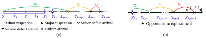
Figure 1.
(a) Corrective replacement happens in $({{S}_{{{A}_{n}}+i}},{{S}_{{{A}_{n}}+i+1}})$; (b) Corrective replacement is taken in $({{S}_{{{A}_{n}}+i+1}},{{S}_{{{A}_{n}}+i+1}}+\tau )$
where $j=0, 1,\cdots , i$;$n=0, 1,\cdots $; $i=0, 1,\cdots ,{{N}_{n+1}}-1$; and ${{N}_{n+1}}={{A}_{n+1}}-{{A}_{n}}$. To ensure that the lower limit of integration is no less than 0, $\Delta (x)$ is defined:
(2) Corrective replacement is taken in $({{S}_{{{A}_{n}}+i+1}},{{S}_{{{A}_{n}}+i+1}}+\tau )$. The severe defective stage is identified by inspection at ${{S}_{{{A}_{n}}+i+1}}$, but the replacement is arranged at the next OM because the time to the next OM is less than the threshold $t$. However, the system fails before the arrival of the next OM.
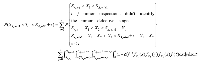
where $f(\tau )$ denotes the pdf of $\tau .$
(3) Corrective replacement is implemented in $({{S}_{{{A}_{n}}+m}},{{S}_{{{A}_{n}}+m+1}}).$ Before the failure arrival, the minor defective stage is identified by inspection at ${{S}_{{{A}_{n}}+n+1}}$. Then, shorter inspection intervals may be adopted. However, the system fails directly after entering the severe defective stageas shown in Figure 2(a).
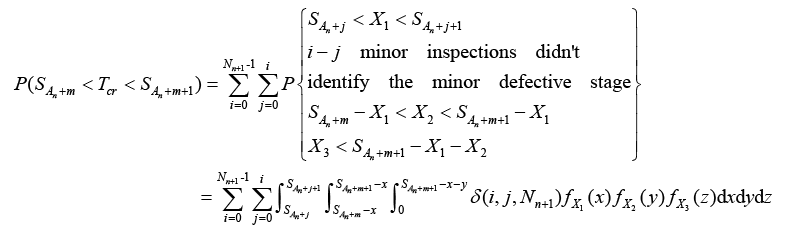
Figure 2.
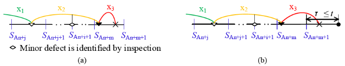
Figure 2.
(a) Corrective replacement is implemented in $({{S}_{{{A}_{n}}+m}},{{S}_{{{A}_{n}}+m+1}})$; (b)Corrective replacement is performed in $({{S}_{{{A}_{n}}+m+1}},{{S}_{{{A}_{n}}+m+1}}+\tau )$
Where $m=i+1, i+2,\cdots $, and $\delta (i, j,{{N}_{n+1}})$ is defined as:
Where $i={{N}_{n+1}}-1$ denotes the inspection implemented at ${{S}_{{{A}_{n}}+i+1}}$ is a major inspection, which can identify the minor defective stage perfectly. While $i<{{N}_{n+1}}-1$, the minor inspection performed at ${{S}_{{{A}_{n}}+i+1}}$can distinguish the minor defective stage with a certain probability $\alpha $.
(4) Corrective replacement is performed in $({{S}_{{{A}_{n}}+m+1}},{{S}_{{{A}_{n}}+m+1}}+\tau ).$Both the minor and severed efective stages are identified by inspections. It is decided to postpone replacement until the next OM since $\tau <t.$As Figure 2(b) shows, in this case, the system fails while waiting for the next OM.
3.2. Probability of Inspection Replacement
When the severe defective stage is identified by inspection, inspection replacement is implemented immediately if the time to the next OMis greater than the threshold t. Depending on whether the minor defective stage isidentified, two situations are discussed.
(1) Inspection replacement happens at ${{S}_{{{A}_{n}}+i+1}}$, as shown in Figure 3(a), and the minor defective stage is not detected by either inspection before implementing the inspection replacement.
Figure 3.
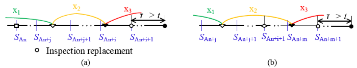
Figure 3.
(a) Inspection replacement happens at ${{S}_{{{A}_{n}}+i+1}}$; (b) Inspection replacement istaken at ${{S}_{{{A}_{n}}+m+1}}$
(2) Inspection replacement is taken at ${{S}_{{{A}_{n}}+m+1}}$. Before the system enters the severe defective stage, the minor defective stage is identified in Figure 3(b).
3.3. Probability of Opportunistic Replacement
If the severe defective stage is identified and the time to the next OM is less than the threshold t, instead of replacing the system immediately, the inspection is stopped and replacement is postponed to the next OM. Then, the opportunistic replacement is implemented successfully before the arrival of failure.
(1) Opportunistic replacement is implemented at ${{S}_{{{A}_{n}}+i+1}}+\tau ,$as Figure 4 (a) shows, and only the severe defective stage is identified by inspection.
Figure 4.
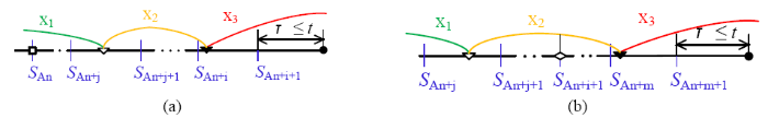
Figure 4.
(a) Opportunistic replacement is implemented at ${{S}_{{{A}_{n}}+i+1}}+\tau $; (b) Opportunistic replacement is performed at ${{S}_{{{A}_{n}}+m+1}}+\tau $
(2)Opportunistic replacement is performed at ${{S}_{{{A}_{n}}+m+1}}+\tau ,$after both the minor and severe defective stages are identified, the system is replaced at OM as shown in Figure 4 (b).
3.4. The Long Run Expected Cost per Unit Time
The probabilities of the system being replaced under different scenarios have been formulated. Then, the expected replacement cycle cost and the expected replacement cycle length of the system need to be expressed to obtain the long run expected cost per unit time.
In order to obtain the expected replacement cycle cost, the expected replacement cycle costs under different replacement scenarios are given first.
(1) When the maintenance action is corrective replacement, the expected replacement cycle cost $E({{C}_{cr}})$ can be expressed as
Where $h(x,{{A}_{n}})$ is defined as
where ${{A}_{n}}=\sum\limits_{k=0}^{n}{{{N}_{n}}}$ and ${{N}_{0}}=0$. ${{N}_{n}}(n=1, 2,\cdots )$ is derived from$N=\left\{ {{N}_{1}},{{N}_{2}},\cdots \right\}$. $N$ is a set of sequential numbers, which mean how many minor inspections are implemented between two major inspections.
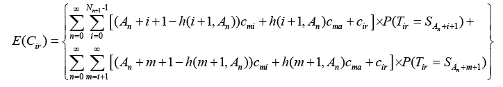
(2) When inspection replacement happens, the expected replacement cycle cost $E({{C}_{ir}})$ is given by
(3) If opportunistic replacement is implemented, the expected replacement cycle cost $E({{C}_{or}})$is
Then, the expected replacement cycle lengths of the system under different replacement scenarios are also formulated.
(1) When the maintenance action is corrective replacement, the expected replacement cycle length $E({{L}_{cr}})$ can be expressed as
(2) When inspection replacement happens, the expected replacement cycle length $E({{L}_{ir}})$ is given by
(3) If opportunistic replacement is implemented, the expected replacement cycle length $E({{L}_{or}})$is
Based on the known expected replacement cycle cost and expected replacement cycle length of the system, the long run expected cost per unit time can be obtained.
where $T=\left\{ {{T}_{1}},{{T}_{2}},\cdots \right\}$ and $N=\left\{ {{N}_{1}},{{N}_{2}},\cdots \right\}$. If the optimal $T,$$N,$ and $t$ can be solved, the minimum long run expected cost per unit time will be obtained. The method to search for optimal decision variables will be studied in future works.
4. Some SpecialCases of this Model
For comparison, some simpler PM models are given. These simpler models are special cases of the proposed model, which can be presented by adopting specific parameters or decision variables. Furthermore, the generality of the proposed model is proven by discussing these special cases.
4.1. Periodic Inspection Model (Model 1)
First, the model proposed in literature [11] (Model 1) is introduced. The system is also subject to minor and major inspections. Both minor and major inspections are periodic inspections. The minor inspection interval is $T$ before the defective stage is identified, i.e.${{T}_{k}}=T,$${{S}_{k}}=kT,\text{ }(k=1, 2,\cdots , i)$. Once the system is found in the minor defective stage at $iT(iT={{S}_{i}})$, the next minor inspection interval is cut to $T/2$, i.e.${{T}_{k}}=T/2,\text{ }(k>i)$.The major inspection interval is $NT$ or $N(T/2)$, which is $N$ times the minor inspection interval, i.e.${{N}_{k}}\equiv N,\text{ }(k=1, 2,\cdots )$. The other assumptions are the same as the proposed model.$T,$$N,$ and $t$ are taken as decision variables for Model 1. In literature [11], the optimal solutions of Model 1 are solved: ${{T}^{\text{*}}}\text{=}4$, ${{N}^{\text{*}}}\text{=}3$, and ${{t}^{\text{*}}}\text{=}2$.
4.2. Sequential Inspection Model without Imperfect Inspection(Model 2)
Due to its lowcost, imperfect inspectionis adopted in this paper. The minor inspection is imperfect inspection, which can identify the minor defective stage with a certain probability but can detect both the normal and severe defective stages perfectly. Substituting perfect inspection for imperfect inspection, a sequential inspection model without imperfect inspection (Model 2) is obtained. In Model 2, inspections can always identify the state of the system perfectly and there is no difference in inspection cost, i.e. $\alpha =1$ and ${{c}_{mi}}={{c}_{ma}}$. The decision variables of Model 2 are $T$ and $t$.
4.3. Sequential Inspection Model Without Postponed Maintenance and OM (Model 3)
When the threshold $t=0$, postponed maintenance and OM will never happen, and a sequential inspection model without postponed maintenance and OM (Model 3) is obtained. For Model 3, only inspection replacement or corrective replacement is implemented. Once the system is found in the severe defective stage, it will be replaced immediately. Formulas of Model 3 canbederived by simplifying the equations established in Section 3. The decision variables of Model 3 are $T$ and $N$.
5. Numerical Example
Inthissection, numerical examples are provided to explain the utility of this model.First, distributions of each stage of the system and parameters are given. Then, a comparison with other models proposed in Section 4 is made to demonstrate the economy of this model. Last, a simple parameters analysis is given to discuss the influence of parameters on the long run expected cost per unit time.
Tomake comparison easier, most of the pdfs and parameters are quoted from literature [11] in this numerical example. Accordingly, it is assumed that the three stages in the gradual degradation process follow three Wei bull distributions, and their pdfs are
Where ${{\lambda }_{n}}$ arescale parameters and ${{k}_{n}}$ are shape parameters $(n=1, 2, 3)$. Parameters used in this numerical example are listed in Table 2.
Table 2. Parameters used in numerical example
| ${{\lambda }_{1}}$ | 15.83 | ${{k}_{1}}$ | 1.47 |
|---|---|---|---|
| ${{\lambda }_{2}}$ | 9.61 | ${{k}_{2}}$ | 1.95 |
| ${{\lambda }_{3}}$ | 6.02 | ${{k}_{3}}$ | 2.81 |
| $\alpha $ | 0.4 | ${{c}_{mi}}$ | 8 |
| ${{c}_{ma}}$ | 20 | ${{c}_{cr}}$ | 3000 |
| ${{c}_{ir}}$ | 400 | ${{c}_{or}}$ | 200 |
| ${{T}_{om}}$ | 200 |
A set of specific decision variables are given to demonstrate the economy of this model. It is noted that these specific decision variables are not the optimal solutions. However, if it is proven that the proposed model is more cost-effective than other models even though the solutions are not the optimal ones, the economic advantage will be more obvious when optimal solutions are solved. Solving optimal solutions of the proposed model is a difficult problem that will be studied in future works.It is supposed that $T$ and $N$ are two specific sequences, which satisfy the following conditions:$T=\left\{ {{T}_{1}},{{T}_{2}},\cdots ,{{T}_{k}},{{T}_{k+1}},\cdots \right\},\text{ }(k=1, 2,\cdots )$:${{T}_{k+1}}\text{=}\left\{ \begin{matrix} {{T}_{k}}\cdot {{T}_{q}}, & {{T}_{k}}\cdot {{T}_{q}}>{{T}^{0}} \\ {{T}^{0}}, & {{T}_{k}}\cdot {{T}_{q}}\le {{T}^{0}} \\ \end{matrix} \right.$(20) Where ${{T}_{q}}$ and ${{T}^{0}}$ are predetermined constants. ${{T}_{q}}$ can be considered the common ratio, and ${{T}^{0}}$ is the lower bound of this sequence. Once ${{T}_{1}}$, ${{T}_{q}}$, and ${{T}^{0}}$ are known, the whole sequence $T$ is defined.Similarly,$N=\left\{ {{N}_{1}},{{N}_{2}},\cdots ,{{N}_{k}},{{N}_{k+1}},\cdots \right\},\text{ }(k=1, 2,\cdots )$:${{N}_{k+1}}=\left\{ \begin{matrix} {{N}_{k}}-{{N}_{d}}, & {{N}_{k}}-{{N}_{d}}>{{N}^{0}} \\ {{N}^{0}}, & {{N}_{k}}-{{N}_{d}}\le {{N}^{0}} \\ \end{matrix} \right.$(21)Where ${{N}_{d}}$ and ${{N}^{0}}$ are also predetermined constants.${{N}_{d}}$ can be considered the common difference, and ${{N}^{0}}$ is the lower bound of $N$. Once ${{N}_{1}}$,${{N}_{d}}$, and ${{N}^{0}}$ are given, the whole sequence $N$ is defined as well. Based on adopting the above specific sequences, a comparison between the proposed model and others model is presented. Decision variables adopted in this example are given in Table 3. Model 1 takes the optimal solution that is solved in paper [11]. Aside from this, the decision variables of other models remain consistent with those of the proposed model. A simulation algorithm is designed to code the whole PM model, and the results under various minor inspection intervals are obtained by many enumerations.
Table 3. Decision variables adopted in example
| $t$ | ${{N}_{1}}(N)$ | ${{N}_{d}}$ | ${{T}_{q}}$ | ${{N}^{0}}$ | ${{T}^{0}}$ | |
|---|---|---|---|---|---|---|
| Proposed model | 2 | 10 | 1 | 0.8 | 3 | 2 |
| Model1 | 2 | 3 | -- | -- | -- | -- |
| Model2 | 2 | -- | -- | 0.8 | -- | 2 |
| Model3 | 0 | 10 | 1 | 0.8 | 3 | 2 |
As illustrated in Figure 5, the abscissa stands for the first item $({{T}_{1}})$ of the minor inspection intervals sequence $T$ (for the proposed model and Model 2) or the inspection interval $T$ of Model 1. The ordinate is the long run expected cost per unit time. The result reveals that the proposed model is more cost-effective than others, even though $T$ and $N$ are not the optimal solutions. This economic benefit may result from the following facts: 1) In the early operation period, the system in the normal stage is a high probability event, and longer inspection interval can save costs. After a period of operation, shortening the inspection interval along with increasing the runtime could prevent unexpected failure. 2) The benefit of taking low-cost imperfect inspection is believed to outweigh the risk that the minor defective stage cannot be identified perfectly by imperfect inspection. The comparison between Model 3 and the proposed model is discussed in the next simulation, where the effect of ${{T}_{OM}}$ and $t$on the long run expected cost per unit time is also presented.
Figure 5.
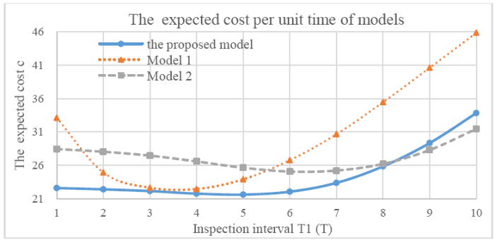
Figure 5.
Comparison between the proposed model and other models
InTable 4, ${{c}^{*}}$ is the minimum long run expected cost per unit time when$T$ and $N$ are the specific sequences. $T_{1}^{*}$ is the first item of the specific minor inspection intervals sequence that minimizes the long run expected cost per unit time. When the threshold $t=0$, the special case Model 3 is obtained. Comparing with the proposed model discussed in the previous example $({{T}_{OM}}\text{=}200,\text{ }t=2)$, it appears that introducing postponed maintenance and OM can generate a very limited economic benefit. However, the cycle length of OM is usually shorter than the expected life cycle length of the system in the practical industry. For example, the refueling cycle length of the reactor is about a year, which would lead to an OM for other equipment in the nuclear power plant. Generally speaking, the expected life cycle length of the equipment is usually longer than one year in nuclear power plants. ${{T}_{OM}}\text{=}200$ Means the OM interval is much longer than the expected life cycle length of the system in this simulation.Therefore, a discussion is made to present the effect of ${{T}_{OM}}$ on the long run expected cost per unit time.As Table 4 shows, the cost is reduced gradually as the OM interval decreases. It is rational to consider that introducing postponed maintenance and OM could be an effective method to improve the economic performance.
Table 4. The effect of ${{T}_{OM}}$ and $t$ on the expected cost
| ${{T}_{OM}}$ | $t$ | $T_{1}^{*}$ | ${{c}^{*}}$ | ${{T}_{OM}}$ | $t$ | $T_{1}^{*}$ | ${{c}^{*}}$ |
|---|---|---|---|---|---|---|---|
| 200 | 0 | 5 | 21.6327 | 150 | 2 | 5 | 21.5905 |
| 1 | 21.5926 | 100 | 5 | 21.5744 | |||
| 2 | 21.5767 | 50 | 5 | 21.5149 | |||
| 3 | 21.6317 | 40 | 5 | 21.4559 | |||
| 4 | 21.8111 | 30 | 5 | 21.4215 | |||
| 5 | 22.0624 | 20 | 5 | 21.3141. | |||
| 10 | 24.3215 | 10 | 4 | 20.8560 |
6. Conclusions
A PM model is proposed for a system subject to a three-stage failure process. In the proposed model, two-level sequential inspections, postponed maintenance and OM, are considered. It is assumed that the failure process of system can be divided into three independent stages: normal, minor defective, and severe defective stages. Considering that the inspection interval changing with the running time of the system would be more cost-effective, two-level sequential inspections are introduced. The minor inspection is a low-cost imperfect inspection that can identify the minor defective stage with a certain probability but can identify the other two stages completely. The major inspection is a perfect inspection that can distinguish the states of the system perfectly. When the system is found in the severe defective stage, it should be replaced immediately if the time to the next OM is greater than a threshold level; otherwise, the replacement is postponed to the next OM. Different replacement situations are studied, and the probabilities of them are derived. Based on this, the expected replacement cycle cost and expected replacement cycle length of the system are obtained, and thus the long run expected cost per unit time is known. Then, some other models are discussed, and these models are special cases of the proposed model and can be obtained by adopting specific parameters or decision variables. In the end, comparison with other models and simple parameters analysis are given to demonstrate the utility of this model in numerical examples. The simulation results demonstrate that there is at least a set of solutions that make the proposed model more economical than other simpler models, even though the solutions are not the optimal ones.
There are several further research topics left for future works based on this paper. First, the optimal solution can be searched to acquire more economic benefits. Second, if the system is found in the minor defective stage by either inspection, more actions can be taken to improve the economic performance, such as preparing maintenance in advance to reduce maintenance cost. Third, the long run expected cost per unit time is selected as a measure tooptimize decision variables in this paper. However, availability is also a remarkable measure besides cost in practice. Therefore, the proposed model could be translated to a new model that can be measured in terms of availability.
Acknowledgements
This work was supported by the National Natural Science Foundation of China (No. 71801141), National Science and Technology Major Project of China (No. ZX069), and Tsinghua University Initiative Scientific Research Program (No. 20151080380).
Reference
“A Summary of Maintenance Policies for a Finite Interval, ”
DOI:10.1016/j.ress.2007.04.004
URL
[Cited within: 3]

It would be an important problem to consider practically some maintenance policies for a finite time span, because the working times of most units are finite in actual fields. This paper converts the usual maintenance models to finite maintenance models. It is more difficult to study theoretically optimal policies for a finite time span than those for an infinite time span. Three usual models of periodic replacement with minimal repair, block replacement and simple replacement are transformed to finite replacement models. Further, optimal periodic and sequential policies for an imperfect preventive maintenance and an inspection model for a finite time span are considered. Optimal policies for each model are analytically derived and are numerically computed.
“Problem Identification in Maintenance Modelling: A Case Study, ”
DOI:10.1080/00207540600960708
URL
[Cited within: 1]
This paper is concerned with a problem identification and problem focus process in maintenance modelling. It endeavours to describe the process of moving from vague problem understanding towards more specific problem formulation and problem focus in the pursuit of practical decision making. This process was conducted using several analytical tools that complemented each other such as regression analyses, snapshot modelling and delay time modelling. As in many case studies related to maintenance modelling, this study also makes use of the experience of experts. It can be seen from the paper that subjective data estimates can prove to be a useful input for modelling. The analysis shows how simple modelling of maintenance problems can provide useful insights and better understanding of the problem in hand.
“A Maintenance Study of Fishing Vessel Equipment using Delay‐Time Analysis, ”
DOI:10.1108/13552510110397421
URL
[Cited within: 1]
The current practice of maintenance on fishing vessels varies according to the operating policies of the owner/operator. On most occasions, the crew does not carry out regular maintenance while at sea. As such, all maintenance work is completed while the vessel is at the discharging port. The time between discharge ports can be as long as three to six months, which allows for failures on the machinery propagating and leading to a catastrophic breakdown. Discusses the possibility of avoiding such events by means of implementing an inspection regime based on the delay-time concept. Operating and failure data that have been gathered from a fishing vessel are used to demonstrate the proposed approach. The outcome of the model is incorporated into the existing maintenance policy of the fishing vessel to assess its effectiveness.
“An Inspection Model based on a Three-Stage Failure Process, ”
DOI:10.1016/j.ress.2011.03.003
URL
[Cited within: 2]
Inspection or condition monitoring is increasingly used in industry to identify the plant item's state and to make maintenance decisions. This paper discusses an inspection model that is established under an assumption that the plant item's state can be classified into four states corresponding to a three-stage failure process. The failed state is always observed immediately, but the other three states, namely normal, minor defective and severe defective, can only be identified by an inspection. The durations of the normal, minor defective and severe defective states constitute a three-stage failure process. This assumption is actually motivated by real world observations where the plant state is often classified by a three colour scheme, e.g., green, yellow and red corresponding to the three states before failure. The three-stage failure concept proposed is an extension to the delay time concept where the plant failure process is divided into a two-stage process. However such extension provides more modelling options than the two-stage model and is a step closer to reality since a binary description of the plat item's state is restrictive. By formulating the probabilities of defective state identification and failure, we are able to establish a model to optimise the inspection interval with respect to a criterion function of interest. A real world example is presented to show the applicability of the model.
“Reducing Production Downtime using Delay-Time Analysis, ”
DOI:10.2307/2581797
URL
[Cited within: 1]
This paper reports on a study in which delay-time analysis and snapshot modelling are jointly applied to model the downtime consequences of a high-speed production line maintained under an inspection system. It is seen that the model is capable of producing results in acceptable agreement with observation and, further, that the technique can be used to predict an efficient inspection frequency for existing plant and also for modified plant yet to be installed.
“Delay-Time Model of Reliability of Equipment Subject to Inspection Monitoring, ”
DOI:10.2307/2582056
URL
[Cited within: 1]
A model is developed for the reliability of a single component, subject to one type of inspectable defect, which will subsequently lead to a failure. Inspections are assumed perfect. The model utilizes the notion of delay time to establish the reliability consequences of inspecting on different inspection periods. The argument is readily extended to the case of a component with multiple and independent defects. Numerical examples are provided.
“An Overview of the Recent Advances in Delay-Time-based Maintenance Modelling, ”
DOI:10.1016/j.ress.2012.04.004
URL
[Cited within: 1]
78 Reviewed the recent advances in delay-time-based maintenance models and applications. 78 Compared the delay-time-based models with other models. 78 Focused on methodologies and applications. 78 Pointed out future research directions.
“Optimal Policies for a Delay Time Model with Postponed Replacement, ”
DOI:10.1016/j.ejor.2013.06.038
URL
[Cited within: 1]
We develop a delay time model (DTM) to determine the optimal maintenance policy under a novel assumption: postponed replacement. Delay time is defined as the time lapse from the occurrence of a defect up until failure. Inspections can be performed to monitor the system state at non-negligible cost. Most works in the literature assume that instantaneous replacement is enforced as soon as a defect is detected at an inspection. In contrast, we relax this assumption and allow replacement to be postponed for an additional time period. The key motivation is to achieve better utilization of the system useful life, and reduce replacement costs by providing a sufficient time window to prepare maintenance resources. We model the preventive replacement cost as a non-increasing function of the postponement interval. We then derive the optimal policy under the modified assumption for a system with exponentially distributed defect arrival time, both for a deterministic delay time and for a more general random delay time. For the settings with a deterministic delay time, we also establish an upper bound on the cost savings that can be attained. A numerical case study is presented to benchmark the benefits of our modified assumption against conventional instantaneous replacement discussed in the literature.
“A Two-Phase Inspection Model for a Single Component System with Three-Stage Degradation, ”
DOI:10.1016/j.ress.2016.10.005
URL
61A two-phase inspection model is studied.61The failure process has three stages.61The delayed replacement is considered.
“A Preventive Maintenance Model with a Two-Level Inspection Policy based on a Three-Stage Failure Process, ”
DOI:10.1016/j.ress.2013.08.007
URL
[Cited within: 5]
61The system′s deterioration goes through a three-stage process, namely, normal, minor defective and severe defective.61Two levels of inspections are proposed, e.g., minor and major inspections.61Once the minor defective stage is found, instead of taking a maintenance action, a shortened inspection interval is recommended.61When the severe defective stage is found, we delay the maintenance according to the threshold to the next PM.61The decision variables are the inspection intervals and the threshold to PM.
“A Delay Time Model for a Mission-based System Subject to Periodic and Random Inspection and Postponed Replacement, ”
DOI:10.1016/j.ress.2016.01.016
URL
61A delay time model of inspection is introduced for mission-based systems.61Periodic and random inspections are performed to check the state.61Replacement of the defective system at a random inspection can be postponed.
“A Condition-based Maintenance Model for a Three-State System Subject to Degradation and Environmental Shocks, ”
DOI:10.1016/j.cie.2017.01.012
URL
[Cited within: 1]
Condition-based maintenance (CBM) is a key measure in preventing unexpected failures caused by internal-based deterioration and external environmental shocks. This study proposes a condition-based maintenance policy for a single-unit system with two competing failure modes, i.e., degradation-based failure and shock-based failure. The failure process of the system is divided into three states, namely, normal, defective and failed, and a defective state incurs a greater degradation rate than a normal state. Random shocks arrive according to a non-homogenous Poisson process (NHPP), leading to the failure of the system immediately. The occurrence of external shocks will be affected to the degradation level of the system. Periodic inspections are performed to measure the state and the degradation level of the system, and two preventive degradation thresholds are scheduled depending on the system state. The expected cost per unit time is derived through the joint optimization of the two preventive thresholds as well as the periodic inspection interval. A numerical example is proposed to illustrate the maintenance model.
“A Summary of Periodic and Random Inspection Policies, ”
DOI:10.1016/j.ress.2010.03.012
URL
[Cited within: 1]
Some systems work for a job with random working times. It would be useful for such systems that they are checked at the completion of working times to detect their failures, which is called a random inspection policy. Two inspection policies, where a system is checked at periodic or successive times and also at every completion of working times, are considered. The total expected costs until the detection of failure are obtained, and when the random working time is exponential, optimal inspection policies which minimize them are derived analytically. Furthermore, the inspection policy where the system is checked only at every completion of N th working time is proposed. Finally, as one of modified random inspection models, the backup model where the system goes back to the latest checking time when it has failed is taken up and analyzed, by using the inspection policy.
“Periodic Inspection Optimization Models for a Repairable System Subject to Hidden Failures, ”
DOI:10.1109/TR.2010.2103596
URL
This paper proposes a model to find an optimal periodic inspection interval over finite and infinite time horizons for a multi-component repairable system subject to hidden failures. The components' failures can only be rectified at periodic inspections, when a failed component is either minimally repaired, or replaced with some age dependent probabilities. We calculate the excepted cost with delayed replacement or minimal repair of a component. Recursive procedures are developed to calculate probabilities of failures in every interval, expected number of minimal repairs, and expected downtimes for optimization over finite and infinite time horizons. Numerical examples of the calculation of the optimal inspection frequencies are given. The data used in the examples is adapted from a hospital's maintenance data for a general infusion pump.
Jardine, “Periodic Inspection Optimization Model for a Complex Repairable System, ”
DOI:10.1016/j.ress.2010.04.003
URL
This paper proposes a model to find the optimal periodic inspection interval on a finite time horizon for a complex repairable system. In general, it may be assumed that components of the system are subject to soft or hard failures, with minimal repairs. Hard failures are either self-announcing or the system stops when they take place and they are fixed instantaneously. Soft failures are unrevealed and can be detected only at scheduled inspections but they do not stop the system from functioning. In this paper we consider a simple policy where soft failures are detected and fixed only at planned inspections, but not at moments of hard failures. One version of the model takes into account the elapsed times from soft failures to their detection. The other version of the model considers a threshold for the total number of soft failures. A combined model is also proposed to incorporate both threshold and elapsed times. A recursive procedure is developed to calculate probabilities of failures in every interval, and expected downtimes. Numerical examples of calculation of optimal inspection frequencies are given. The data used in the examples are adapted from a hospital's maintenance data for a general infusion pump.
“Periodic Inspection Optimization of a k-out-of-n Load-Sharing System, ”
DOI:10.1109/TR.2015.2421819
URL
[Cited within: 1]
In this paper, we consider a k-out-of-n load-sharing system with n identical components sharing a certain amount of load. Each time a component fails, its load is distributed to the remaining components; we assume an increase in load increases the hazard rates of the remaining components. The system is periodically inspected to detect failed components. Two cases may occur in an inspection interval: if the number of failed components is less than n-k+1, then the failed components are only rectified at periodic inspections; if the number of failures reaches n-k+1, then the system fails, and at this time, all the failed components are inspected and rectified. A failed component is replaced or minimally repaired according to a probability which depends on its age at the failure time. The components' failures follow a Non-Homogenous Poisson Process (NHPP), and their intensity functions depend on their ages and the loads to which they are exposed at any moment. In this paper, we develop a model to find the optimal inspection interval for such a system, which minimizes the total expected cost incurred over the system lifecycle. We derive the analytical solution for the special case of a 1-out-of-2 system, and discuss its computational difficulties. We then present a simulation algorithm to find the required expected values in the objective function. Several numerical examples are presented to illustrate the proposed model.
“Sequential Inspection Strategy for Multiple Systems under Availability Requirement, ”
DOI:10.1016/S0377-2217(02)00822-6
URL
[Cited within: 1]
System failures are usually observed during regular maintenance or inspection and this is especially the case for systems in standby or storage, which is common for safety critical systems. A periodic inspection policy is usually adopted. However, during the inspection, a lot of information is gained about the status of the system. Such information should be used in deciding upon the time for the next inspection. Hence sequential inspection is more appropriate, especially when the aging property of the system is unknown, and has to be estimated with the information from inspection. In this paper, a model is developed and sequential inspection strategies are studied in this situation. The focus is on the case when there are multiple systems inspected at the same, but discrete times. We also do not assume a known distribution of the system life time, and the estimation of that is incorporated into the analysis and decision making. Different availability criteria are considered and numerical examples are provided to illustrate the procedure.
“Optimization of Alarm Threshold and Sequential Inspection Scheme, ”
DOI:10.1016/j.ress.2009.09.012
URL
[Cited within: 1]
An item is subject to gradual degradation. The degradation can be represented by a measurable, non-negative and non-decreasing quantity. The item can be in one of three different states: normal (when the degradation quantity is smaller than a threshold of alarm or potential failure), functional failure (when the degradation quantity is larger than a functional failure threshold) and in-between or potential failure (when the degradation quantity is larger than the alarm threshold and smaller than the functional failure threshold). A sequential inspection scheme is implemented to determine the state of the item so as to prevent a functional failure. The paper presents a flexible degradation model and two cost models to optimize the alarm threshold and the sequential inspection scheme. The usefulness and appropriateness of the proposed models are illustrated by examples.
“Simple Method for Risk Assessment of Nuclear Power Plant Refueling Outages, ”
DOI:10.1016/s0029-5493(96)01190-9
URL
[Cited within: 1]
This paper discusses the method used for probabilistic risk assessment (PRA) studies of the Monticello Nuclear Power Plant's 1993 and 1994 refueling outages. The method made full use of work already completed as part of the United States Nuclear Regulatory Commission's request for at-power risk studies known as individual plant examinations (IPEs) and therefore required less resources than many other techniques for shut-down risk management. The four plant models used to examine various plant outage states are described and discussed. The models are (1) reactor during manual shut-down, (2) reactor in cold shut-down with head installed, (3) reactor with head off and (4) fuel storage pool. These models were manipulated before the refueling outage began using the computer programs SETS and CAFTA to simulate different decay heat levels and various components out of service during time segments of the outage. This was used to identify higher risk periods during the outage and to sensitize operators and other personnel to the important equipment and activities during the daily briefings during the outage. Several techniques are discussed in this paper, including (1) methods to modify an existing PRA model for lower decay heat conditions, (2) editing existing cutsets to simulate various equipment availability states and (3) the use of assumptions to simplify the analysis
Cavalcante, “A Study of Postponed Replacement in a Delay Time Model, ”
