


1.Introduction
At present, the method of fault diagnosis can be divided into the method based on mechanism modeling, the method based on knowledge engineering, and the data driven method [1]. The vibration signals of therolling bearing have complex coupling and nonlinearity. Traditional fault diagnosis usually cannot deeply dig data and lacks the related technology to improve the data application.
Empirical Mode Decomposition (EMD) is a time-frequency analysis method proposed by Huang in 1998. EMD has been rapidly developed and widely usedin gearbox fault processing[2-3]. EMD has good adaptability and can be decomposed according to its own characteristics of the fault signal to obtain prominent local features in the intrinsic mode components. However, due to the appearance of modal aliasing, the diagnostic accuracy is affected. EEMD is an improvement ofthe EMD method. Noise-assisted analysis of gearbox fault signals can reduce the effect of modal aliasing and further improve the analysis [4]. The EEMD is an adaptive signal processing method that is well suited for handling nonlinear non-stationary signals. However, in strong noisy environments, the noise often affects the sensitive IMF. The high-frequency weak feature frequencies are easily submerged in the noisy IMF, which is not conducive to fault identification [4]. Some researchers have proposed combining with other classification algorithms for fault diagnosis. References [5-7] combined EEMD and the BP neural network to realize the fault diagnosis of gear and rolling bearing; however, the superficial learning algorithm used has limited ability of expression, which makes it hard to classify high-dimensional and nonlinear features and is apt to fall into the local optimum.
Before the theory of deep learning was proposed, most of the fault recognition techniques were based on a relatively shallow learning structure, which relied on a large amount of signal processing and human experience. However, the model based on deep learning deals with massive data through a multi-hidden network structure model. The neurons in the hidden layer automatically learn the features in the data to obtain more efficient features than artificial selection, thereby removing the dependence on experience and improving the accuracy of classification or prediction. The Deep Belief Network (DBN) has been applied in the field of process monitoring, power grid fault diagnosis, and mechanical equipment fault status recognition in recent years. References [8-9] used the normalized rolling bearing original time-domain signal to train the DBN and completed the fault diagnosis. Reference [10] studied the ball bearing fault diagnosis using a combination of SVD and DBN. Inreference [11], the double-tree complex wavelet and DBN were used to study the classification of bearing fault types, which extended the application of DBN in fault areas. Reference [12] used the EEMD-Hilbert envelop spectrum and DBN to study the state recognition of rolling bearing and achieved good diagnostic results. However, the number of DBN nodes is relatively large, which results in complex structure and long training time and is not conducive to real-time monitoring. DBN consists of several Restricted Boltzmann Machines (RBMs). RBM is constrained by the two values of input nodes, andit cannot be directly appliedin processing data and detecting. Generally, the vibration signal of rolling bearing is a continuous realvalue, while the Gaussian Bernoulli limited Boltzmann machine (GBRBM) can handle the real value data. Therefore, using GBRBM instead of RBM to build the Gaussian Bernoulli depth belief network (GBDBN) can solve the problem that the vibration signal of rolling bearing is a real value. At present, research on using GBDBN for fault diagnosis is limited. However, when GBDBN is affected by disturbing factors, its output has a certain randomness, so it is easy to misclassify the fault classification. As a result, its performance is not stable.
Aiming at the problem that the traditional method cannot recognize high-frequency weak features after EEMD under a strong noise environment, combined with the advantages of GBDBN where it can directly process real-valued data and adaptively mine deep features of high-dimensional data, a new fault diagnosis method of rolling bearing is proposed. The method firstly carries out EEMD on the vibration signal, then determines the characteristics of each IMF, selects the features with smaller changes as the eigenvectors, and inputs them into GBDBN for fault type identification. Experiments show that this method has a beneficial effect.
2. Modeling Method of Fault Diagnosis based on EEMD and GBDBN
Based on EEMD and GBDBN, a fault recognition model for rolling bearings, inner rings, and outer rings of rolling bearings is established, and it is used to determine whether the ball bearings, inner rings, and outer rings of rolling bearings are faulty. The process of rolling bearing fault diagnosis based on EEMD and GBDBN is shown in Figure 1.
Figure 1.
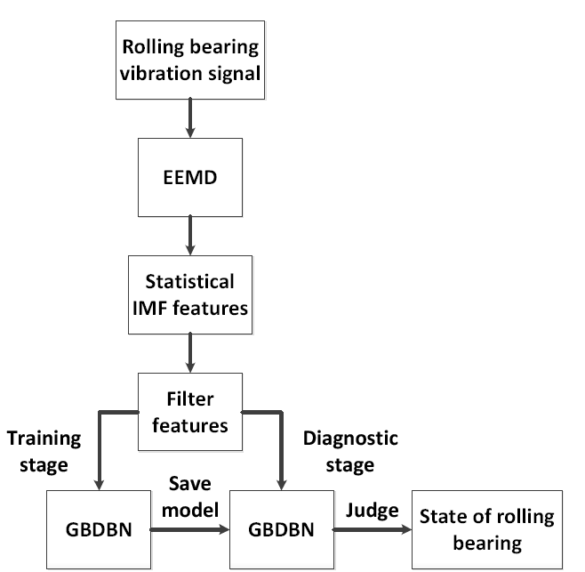
Figure 1.
Fault diagnosis model of rolling bearing based on EEMD and GBDBN
This method first draws on the advantages of EEMD, extracts features from nonlinear vibration signals of rolling bearings, and reduces the influence of non-stationary signals and the interference of uncertain factors. Then, the statistical feature of IMFs is used as the input of GBDBN to reduce the number of nodes of GBDBN. Finally, we use the ability of GBDBN to excavate the deep features of high-dimensional data to identify fault types and finally realize the recognition of several types of faults and different fault states of rolling bearings. The implementation process is as follows:
Training stage:
$\cdot$ The vibration data of the rolling bearing is collected and processed by EEDM to obtain each IMF component;
$\cdot$ Using time-domain statistical methods to calculate each IMF component, obtain the statistical characteristics;
$\cdot$ Select the feature vectors with smaller changes and input them to GBDBN for training;
$\cdot$ The trained model is saved to facilitate the diagnosis of the call.
Diagnostic stage:
$\cdot$ The vibration data of the rolling bearing are collected and processed, and the process is the same as the training stage. Then, the features are extracted;
$\cdot$ The feature vectors are extracted and input into the trained GDDBN for fault identification to determine the state of the rolling bearing.
3. The Principle of EEMD and the Method of Time Domain Statistics
3.1. The Principle of EEMD
$\cdot$ Let the original signal be $x(t)$ and make $N$ the number of polymerization; at the same time, remember $m=1$;
$\cdot$ A new test signal ${{x}_{m}}(t)$ is generated by adding Gaussian white noise with a magnitude factor of $k$ in $x(t)$:
$\cdot$ Using the EMD method, decompose${{x}_{m}}(t)$ into a series of IMFs;
$\cdot$ When $m<N$, steps (2) and (3) are repeated, but the newly added Gauss white noise needs to be distinguished from the previous several times; at the same time, make $m=m+1$;
$\cdot$ After the above decomposition, several groups of IMFs are produced with the mean value of
where $N$ is the number of polymerization and ${{c}_{i, m}}$ is the ith IMF obtained by the $m$ decomposition.
The last EEMD intrinsic mode function is the average of the Nth decomposition of each IMF above.
3.2. The Method of Time Domain Statistics
Signal characteristics reflect the inherent law of the signal and, to a certain extent, are symbolic. Reference [15] pointed out that the advantage of the characteristic parameter method lies in that only a few indicators are required to explain the bearing state. Statistical characteristics of each IMF are calculated as follows:
Average value:
Maximum value:
Peak to peak values:
Root Mean Square:
Kurtosis:
Wave form factor:
Peak factor:
Kurtosis factor:
Pulse factor:
Margin factor:
4. Design and Optimization for Planar-Type Voice Coil Motor
GBDBN is a generation model established by training the weights between the neurons of its layers and the layers, so that the whole model can train the data according to the maximum probability to realize the data type identification or classification [16-21]. The components of GBDBN are GBRBMs and consist of multiple GBRBMs stack by stack. Two neurons in each GBRBM correspond to GBDBN. Receiving data involves the explicit layer, while feature extraction involves the hidden layer. Correspondingly, the neurons in the explicit layer and the hidden layer are the explicit element and the hidden element, respectively. Therefore, the process of training GBDBN is the process of training GBRBM [19,22-23]. In each GBRBM, the explicit layer receives the data to infer the hidden layer and then treats the hidden layer as the explicit layer of the next GBRBM. The explicit element of GBRBM can take a continuous real number, while the hidden element can only take 0 or 1. This feature of GBRBM makes it fit for modeling real value data[10], asshown in Figure 2.
Figure 2.
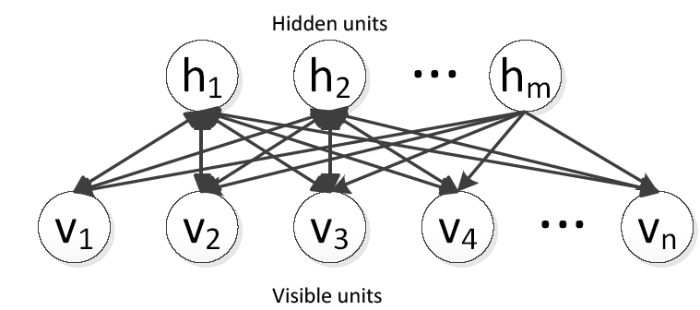
Figure 2.
Composition of RBM
According to reference [3], the system energy function of GBRBM is defined as
Where ${{\sigma }_{i}}$ is the standard deviation of Gaussian noise corresponding to explicit element ${{v}_{i}}$,$\theta =\{{{W}_{ij}},{{a}_{i}},{{b}_{j}}\}$ is the GBRBM structural parameters,${{W}_{ij}}$ represents the connection weight between explicit element ${{v}_{i}}$ and hidden element ${{h}_{j}}$,${{\text{a}}_{i}}$ represents the offset of the explicit element ${{v}_{i}}$,${{\text{b}}_{j}}$ represents the offset of the hidden element ${{h}_{j}}$, andall parameters are real numbers.
Therefore, the joint probability distribution of the explicit and hidden layers is
To simplify the model reasoning, it is necessary to normalize the data in advance of the use of GBRBM. For the training of GBRBM, the learning algorithm of Contrastive Divergence is adopted. The specific operations are described as follows:
$\cdot$ First, the excitation value of each hidden unit is calculated:
$\cdot$ Then, the excitation values of each hidden unit are normalized by the S-shaped function and become the probability value of opening (denoted by 1):
$\cdot$ For the S-shaped function, we use the logistic function as follows:
$\cdot$ So far, the probability in the opening state of each hidden unit is calculated. Thus, the probability in the closing state of each hidden unit (denoted by 0) is
$\cdot$ As to whether the neuron is opened or closed, we need to compare the probability of opening with a random value drawn from a (0, 1) uniform distribution:
$\cdot$ As follows:
Then, open or close the corresponding hidden unit according to the above calculation. Similarly, given the hidden layer, the visible layer can be calculated according to the above calculation.
For training RBM, the algorithm shown as follows is the Contrastive Divergence, proposed by Hinton:
$\cdot$ For each record $x$ in the training set, we assign $x$ to the visible layer ${{v}^{(0)}}$ to compute the probability that the hidden layer neurons are opened:
Where superscripts and subscripts are used to distinguish different vectors and dimensions respectively in the same vector.
$\cdot$ Then, a sample is extracted by using Gibbs sampling from the calculated probability distribution:
$\cdot$ Reconstruct the visible layer with ${{h}^{(0)}}$:
$\cdot$ Likewise, a sample of the visible layer is extracted:
$\cdot$ The probability of neurons in the hidden layer being opened is again calculated using visible layer neurons (after reconstruction):
$\cdot$ The updated weights are as follows:
After sufficient training, GBRBM can accurately implement the feature extraction or reducing feature [21].
The GBDBN consists of multiple GBRBM. To obtain a better training effect, the pre-training process uses the unsupervised greedy method, trains from bottom to top layer by layer, and obtains the parameters of each layer.
$\cdot$ Firstly, fully train the first GBRBM;
$\cdot$ Save the weight and offset obtained after training the first GBRBM, and take the state of its hidden element as the input of the next GBRBM;
$\cdot$ After fully training the current GBRBM, the current GBRBM is stacked above the last GBRBM;
$\cdot$ Repeat the third step any number of times until the top level is reached;
$\cdot$ Train data and label classification on top level GBRBM using classified neurons;
$\cdot$ After the GBDBN is trained, the schematic diagram is shown in Figure 3.
Figure 3.
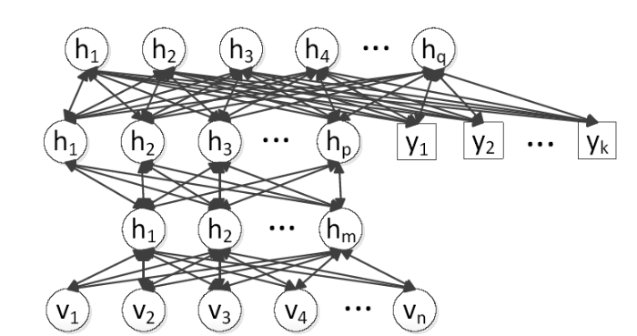
Figure 3.
The schematic diagram of training completed GBDBN
The generation model uses the Contrastive Wake-Sleep algorithm to tune, and the process of the algorithm is as follows:
$\cdot$ In addition to the top-level RBM, the weights of the other RBM are divided into an upward cognitive weight and a downward generation weight;
$\cdot$ Wake phase: produce an abstract representation of each layer through the external characteristics and the upward weight, and use gradient descent to modify the downward weights between layers;
$\cdot$ Sleep phase: generate the state of next neurons through the top-level neurons of classification and downward weight, and modify the upward weight between the layers.
5. Experiment and Analysis
The experimental data came from the bearing data center of Case Western Reserve University in the United States. In this paper, only a part of the data was selected as an experimental analysis.The model of the rolling bearing is 6205-2RS, and the drive-end accelerometer data is collected at a 12K sampling rate.The speed of the motor is 1730r/min.The damage conditions of the rolling bearings are single damage, manufactured by artificial EDM, and the damage diameter is 0.007 inches, 0.014 inches, and 0.021 inches, respectively.The state of the rolling bearing is divided into normal, inner ring fault, ball fault, and outer ring fault.Among them, the outer diameter of rolling bearing with damage diameter of 0.007 inches includes three faults in the directions of 3 o’clock, 6 o’clock, and 12 o’clock, and the other two kinds of damaged outer diameters of rolling bearing are all in the direction of 6 o’clock.There is a total of 12 working conditions.The sampling time of each sample is 0.1 seconds, so the number of sampling points for each sample is 1200, and the number of samples for each working condition is 100.80 samples of each condition were randomly selected for training and the remaining 20 samples were tested.The data is illustrated as follows. The 0.007 inch outer ring fault 6 indicates that the damage diameter is 0.007 inches, the outer ring fault of the rolling bearing is in the 6 o’clock direction, and the other is the analogy shown in Table 1.
Table 1. Data description of rolling bearings
| States of the rolling bearing | Numbers of training data | Numbers of testing data | Classification label |
|---|---|---|---|
| Normal | 80 | 20 | 1 |
| 0.007-inner-ring-fault | 80 | 20 | 2 |
| 0.007-ball-fault | 80 | 20 | 3 |
| 0.007-outer-ring-fault-6 | 80 | 20 | 4 |
| 0.007-outer-ring-fault-3 | 80 | 20 | 5 |
| 0.007-outer-ring-fault-12 | 80 | 20 | 6 |
| 0.021-inner-ring-fault | 80 | 20 | 7 |
| 0.021-ball-fault-fault | 80 | 20 | 8 |
| 0.021-outer-ring-fault-6 | 80 | 20 | 9 |
| 0.028-inner-ring-fault | 80 | 20 | 10 |
| 0.028-ball-fault -fault | 80 | 20 | 11 |
| 0.028-outer-ring-fault-6 | 80 | 20 | 12 |
Firstly, EEMD is used to process the vibration signals to extract valid information. The results are shown in Figures 4-9. Limited to space, only show the decomposition results of normal signals, and the rolling bearing with damage diameter of 0.007 inches includes three fault of inner ring fault, ball fault, and outer ring fault. IMF1~IMF9 represent the decomposition results from high frequency to low frequency.
Figure 4.
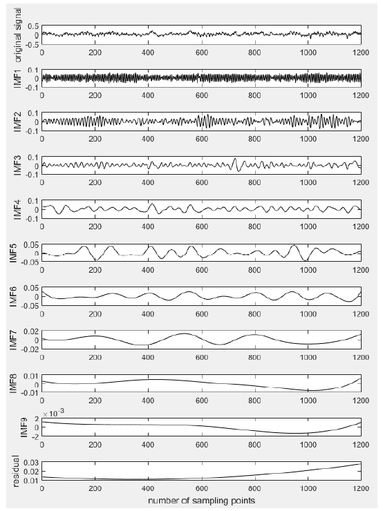
Figure 4.
EEMD diagram of normal vibration signals of rolling bearings
Figure 5.
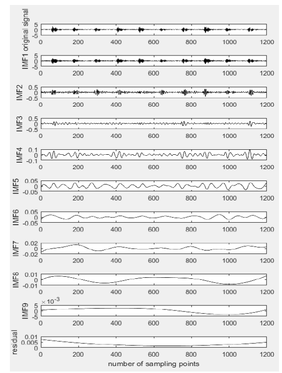
Figure 5.
EEMD diagram of inner-ring-fault vibration signals of rolling bearings
Figure 6.
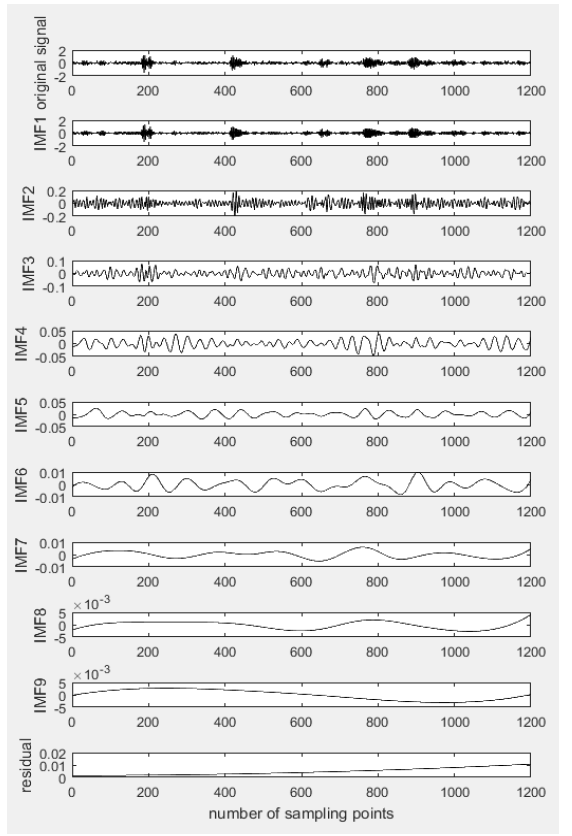
Figure 6.
EEMD diagram of ball-fault vibration signalsof rolling bearings
Figure 7.
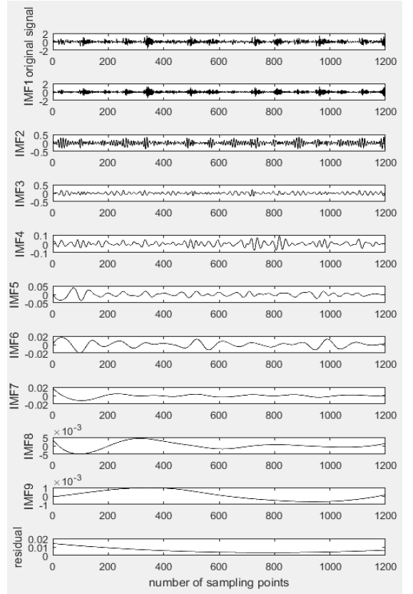
Figure 7.
EEMD diagram of outer-ring-fault 3 o’clock vibration signals of rolling bearings
When the rolling bearing has different faults, the distribution of fault signals in each IMF component will change accordingly, so the statistical feature of different frequency bands should be selected as the feature vectors of fault recognition [17,20,24-26]. The characteristics of each IMF component are calculated according to the formula in Table 1, and the results are shown in Figure 5. Due to space limitations, only some of the features of the normal signal are listed. It can be seen from the figure that the IMF component varies from high frequency to low frequency, and the characteristic values change obviously with a difference of several orders of magnitude. Considering the GBDBN method applied in image recognition, each pixel value of the image varies from 0 to 255, so choose the value of the feature that is not too different and not greater than 255. Thus, the paper selects the kurtosis, peak factor, pulse factor, and margin factor of each IMF component as the input of GBDBN.
Figure 8.
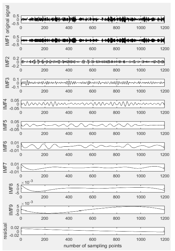
Figure 8.
EEMD diagram of outer-ring-fault 6 o’clock vibration signals of rolling bearings
Figure 9.
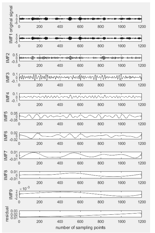
Figure 9.
EEMD diagram of outer-ring-fault 12 o’clock vibration signals of rolling bearings
After feature extraction, each sample contains 36 eigenvectors and their corresponding sample tags, which are input to GBDBN for training. The first hidden layer is trained by using the sample feature vector as the input of GBDBN, then the first hidden layer is used as input layer to train the second hidden layers, and the last layer is the classification layer, which constitutes the whole network. The whole GBDBN has four layers, and the structure is 36-120-100-12, that is, the number of neurons in each layer is 36, 120, 100, and 12, respectively. The experiment training times is 1000.During the training process, there usually will be an overfitting phenomenon, so uses Dropout to prevent over-fitting. For better convergence, the learning rate of the model should not be too large, and it is set to 0.1. To make up for the defect that the derivative form of sigmoid function tends to be saturated, a cross-entropy cost function is introduced.
The data of Table 2 are tested and repeated ten times. The results of the experiment are shown in Table 3. After ten times of diagnostic experiments, the method proposed in this paper has a recognition rate of more than 90% for rolling bearing fault types and has good diagnostic capability. To further analyze the effectiveness of the method proposed in this paper, ten experiments are carried out using the same structure of Back Propagation Neural Network (BPNN) and DBN. The comparison results show that the recognition rate of GBDBN is higher than that of BPNN and DBN, which indicates that GBDBN has better classification ability and learning ability than BPNN and DBN.
Table 2. Part of the IMF’s statistical features
| Feature | IMF1 | IMF5 | IMF9 |
|---|---|---|---|
| Maximum value | 0.066067 | 0.023866 | 0.002001 |
| Average value | 3.337e-05 | -0.00166 | -0.00037 |
| Peak to peak | 0.134285 | 0.051006 | 0.003444 |
| Root mean square root | 0.028894 | 0.012619 | 0.000824 |
| Kurtosis | 1.840338 | 2.110486 | 3.257759 |
| Wave form factor | 865.9293 | -7.61671 | -2.24890 |
| Peak factor | 4.647441 | 4.041924 | 4.178347 |
| Kurtosis factor | 2640199 | 83224912 | 7.057e12 |
| Pulse factor | 5.304240 | 4.703455 | 5.000333 |
| Margin factor | 5.873662 | 5.278838 | 5.684202 |
Table 3. Experimental results
| Number of experiments | Recognition rate of BPNN | Recognition rate of DBN | Recognition rate of GBDBN |
|---|---|---|---|
| 1 | 88.33% | 89.17% | 90.94% |
| 2 | 80.26% | 85.83% | 90.21% |
| 3 | 81.62% | 85.83% | 90.63% |
| 4 | 86.25% | 87.08% | 90.00% |
| 5 | 84.11% | 84.58% | 90.63% |
| 6 | 86.67% | 88.75% | 91.35% |
| 7 | 87.92% | 89.17% | 90.31% |
| 8 | 85.00% | 88.92% | 91.36% |
| 9 | 86.83% | 86.67% | 90.33% |
| 10 | 82.95% | 85.42% | 90.25% |
6. Conclusions
The fault diagnosis method of rolling bearing based on EEMD and GBDBN is proposed in this paper. It combines feature extraction with deep learning and makes the most of the advantages of the EEMD and GBDBN methods. Taking the statistical characteristics of IMFs as the training data of GBDBN and avoiding directly inputting the original signal into the deep neural network training reducesthe number of neurons and the complexity of the deep neural networkto a certain extent and improves the efficiency of diagnosis, resulting inbetter performance for fault diagnosis.Firstly, the whole model of the rolling bearing fault diagnosis based on EEMD and GBDBN is introduced, and then the methods of feature extraction and processing data of EEMD andmodeling method of GBDBN are introduced respectively.Finally, the experiment verifies the effectiveness of the proposed method.Compared with BPNN and DBN, GBDBN has strong ability of data identification and fault diagnosis.To verify the versatility of the method proposed in this paper, we pre-train the data of several types of rolling bearings. The results prove that this method can accurately identify bearing failures.
Acknowledgements
This work was financially supported by the National Natural Science Foundation of China and the Civil Aviation Administration of China Joint Funded Projects (No. U1733108), Tianjin Science and Technology Support Program Key Project (No. 16YFZCSY00860), Natural Science Foundation of Tianjin(No. 17JCQNJC04300),Natural Science Foundation of Tianjin (No. 16JCYBJC18400),and Open Funding of the State Key Laboratory of Mechanical Transmissions (No. SKLMTKFKT-201616).
Reference
“A New Convolutional Neural Network based Data-Driven Fault Diagnosis Method, ”
DOI:10.1109/TIE.2017.2774777
URL
[Cited within: 1]

Fault diagnosis is vital in manufacturing system, since early detections on the emerging problem can save invaluable time and cost. With the development of smart manufacturing, the data-driven fault diagnosis becomes a hot topic. However, the traditional data-driven fault diagnosis methods rely on the features extracted by experts. The feature extraction process is an exhausted work and greatly impacts the final result. Deep learning (DL) provides an effective way to extract the features of raw data automatically. Convolutional neural network (CNN) is an effective DL method. In this study, a new CNN based on LeNet-5 is proposed for fault diagnosis. Through a conversion method converting signals into two-dimensional (2-D) images, the proposed method can extract the features of the converted 2-D images and eliminate the effect of handcrafted features. The proposed method which is tested on three famous datasets, including motor bearing dataset, self-priming centrifugal pump dataset, and axial piston hydraulic pump dataset, has achieved prediction accuracy of 99.79%, 99.481%, and 100%, respectively. The results have been compared with other DL and traditional methods, including adaptive deep CNN, sparse filter, deep belief network, and support vector machine. The comparisons show that the proposed CNN-based data-driven fault diagnosis method has achieved significant improvements.
“Planetary Gearboxes Fault Diagnosis based on EMD and EDT, ”
in
DOI:10.1109/PHM.2015.7380039
URL
[Cited within: 2]

Planetary gearbox is widely used in many fields due to its robustness and high power-weight ratio, but implement fault diagnosis on it is a challenge all the time. This paper proposed a new fault diagnosis method of planetary gearbox based on EMD and EDT. Firstly, the vibration data is decomposed into several IMFs by EMD. Then select sensitive IMFs which contain main fault information depend on the correlation coefficients between IMF and fault, normal signal. At the same time, extract energy of the sensitive IMFs as feature parameter. Finally, implement fault diagnosis used EDT. The effectiveness of this new method is validated by gearbox vibration data obtained from test-rig, and the final diagnosis results show that the technique is accurate and reliable. It is helpful in practical application.
“Condition Recognition Method of Rolling Bearing based on Ensemble Empirical Mode Decomposition Sensitive Intrinsic Mode Function Selection Algorithm, ”
“Gear Defect Detection based on EEMD and BP Neural Networks, ”
Aiming at overcoming the difficulties in noise analysis, such as the complexity of the gear noise signals, and the interference by outside noises, a new noise analysis method was proposed based on ensemble empirical mode decomposition(EEMD)algorithm, time synchronous averaging(TSA)and back propagation(BP)neural network.EEMD was used to extract useful signals from the original signal based on the gear mesh frequency and multiplication of the mesh frequency.TSA was used for further de-noising.Then the feature values of the tested signals after de-noising were calculated.Discriminative features among different gear defect type were selected and taken as the input of BP neural network, the type of gear defect was effectively identified.The results of our experiments indicate that the proposed method based on EEMD and TSA enhances the denoise effect, and effctive features are obtained after the de-noising.Moreover, the inference of the gear defect type based on the BP neural network could avoid the disadvantages of humans' subjective judgments, and achieves accurate identification results.
“Fault Diagnosis Method of Fan Gearbox based on EEMD and BP Neural Network, ”
“Rolling Bearing Fault Diagnosis based on EEMD and Fuzzy BP Neural Network, ”
Considering non-stationary characteristics of bearing's fault vibration signals, an EEMD and fuzzy neural network-based fault diagnosis method was proposed, in which, having EEMD method adopted to decompose the bearing's bearing vibration signals into several intrinsic mode function components(IMF); and then, extracting each component's mean square error, kurtosis and energy and taking them as learning set and training set; and finally, having the learning set input into the fuzzy BP neural network for learning and the training set into the fuzzy BP neural network for fault type identification. Experimental results show that, the method proposed can be effectively applied to the rolling bearing's fault diagnosis and it outperforms the BP neural network in the accuracy.
“Signal Reconstruction and Bearing Fault Recognition based on Deep Belief Network, ”
“Research on Fault Feature Extraction and Diagnosis Method based on DBN, ”
“A Fault Diagnosis Method for Rolling Bearings based on Singular Value Decomposition and Deep Belief Network, ”
“Fault Diagnosis of Bearing based on Dual Tree Complex Wavelet and Deep Belief Network, ”
“State Identification Method of Rolling Bearings based on EEMD-Hilbert Envelope Spectrum and DBN Variable Loads, ”
The load usually is changing during the running process of the rolling bearing. Aiming at the multiple-state recognition difficult problem of different fault locations and different performance degradation degrees for rolling bearing under variable load, based on ensemble empirical mode decomposition-Hilbert(EEMD-Hilbert) envelope spectrum and deep belief network(DBN), a state recognition method of a rolling bearing is proposed. At first, the vibration signals of each state of the rolling bearing are decomposed by EEMD. Then, the sensitive intrinsic mode function(IMF) components of each signal are selected and their envelope spectrum can be obtained using Hilbert transform. At last, the new high-dimensional data can be constructed by IMF envelope spectrum of each state vibration signal according to certain order, and then the new high-dimensional data are used as the input of DBN, whose each hidden layer node structure had been optimized using genetic algorithm, and multiple-state recognition of the rolling bearing under variable load can be achieved. The experimental results show that, by using DBN, during the recognition process of the 10 states of the rolling bearing, if training data choose a certain load and testing data choose another load, the multiple-state feature of rolling bearing under different loads can be reflected better by using EEMD-Hilbert envelope spectrum than the time domain or frequency domain amplitude spectrum. And, comparing with the shallow learning support vector machine and BP neural network algorithm, DBN has a higher recognition rate and the recognition rate of each data set can reach more than 92.5%.
“Non-Linear Multivariate and Multiscale Monitoring and Signal Denoising Strategy using Kernel Principal Component Analysis Combined with Ensemble Empirical Mode Decomposition Method, ”
DOI:10.1016/j.ymssp.2011.03.002
URL
[Cited within: 1]
The article presents a novel non-linear multivariate and multiscale statistical process monitoring and signal denoising method which combines the strengths of the Kernel Principal Component Analysis (KPCA) non-linear multivariate monitoring approach with the benefits of Ensemble Empirical Mode Decomposition (EEMD) to handle multiscale system dynamics. The proposed method which enables us to cope with complex even severe non-linear systems with a wide dynamic range was named the EEMD-based multiscale KPCA (EEMD-MSKPCA). The method is quite general in nature and could be used in different areas for various tasks even without any really deep understanding of the nature of the system under consideration. Its efficiency was first demonstrated by an illustrative example, after which the applicability for the task of bearing fault detection, diagnosis and signal denosing was tested on simulated as well as actual vibration and acoustic emission (AE) signals measured on purpose-built large-size low-speed bearing test stand. The positive results obtained indicate that the proposed EEMD-MSKPCA method provides a promising tool for tackling non-linear multiscale data which present a convolved picture of many events occupying different regions in the time requency plane.
“The Empirical Modal Decomposition and Fuzzy Entropy Feature Analysis of Fault Signals of High Speed Train Bogies, ”
“Vibration Detection Method of Rolling Bearing Fault, ”
“Research on Bearing State Recognition based on Deep Learning Theory, ”
“Classification and Recognition of Bearing Faults based on Deep Belief Network, ”
“Method of Health Monitoring of Mechanical Equipment Big Data based on Deep Learning Theory, ”
“Failure Diagnosis using Deep Belief Learning based Health State Classification, ”
DOI:10.1016/j.ress.2013.02.022
URL
[Cited within: 1]
Effective health diagnosis provides multifarious benefits such as improved safety, improved reliability and reduced costs for operation and maintenance of complex engineered systems. This paper presents a novel multi-sensor health diagnosis method using deep belief network (DBN). DBN has recently become a popular approach in machine learning for its promised advantages such as fast inference and the ability to encode richer and higher order network structures. The DBN employs a hierarchical structure with multiple stacked restricted Boltzmann machines and works through a layer by layer successive learning process. The proposed multi-sensor health diagnosis methodology using DBN based state classification can be structured in three consecutive stages: first, defining health states and preprocessing sensory data for DBN training and testing; second, developing DBN based classification models for diagnosis of predefined health states; third, validating DBN classification models with testing sensory dataset. Health diagnosis using DBN based health state classification technique is compared with four existing diagnosis techniques. Benchmark classification problems and two engineering health diagnosis applications: aircraft engine health diagnosis and electric power transformer health diagnosis are employed to demonstrate the efficacy of the proposed approach. (C) 2013 Elsevier Ltd. All rights reserved.
“Gear Box Fault Recognition based on Depth Learning Neural Network, ”
“Dynamic Monitoring of Bearing States based on Multiple Sparse Self Coding, ”
“Fault Diagnosis of Induction Motor based on Sparse Automatic Coding Deep Neural Network, ”
“Research on EEMD-RA-KU Method for Bearing Fault Detection, ”
“Nonlinear Process Fault Detection based on Gauss Restricted Boltzmann Machine, ”
“Gear Intelligent Fault Diagnosis based on Deep Learning Feature Extraction and Particle Swarm Support Vector Machine, ”
“Fault Diagnosis based on Self Encoding Stack Noise, ”
