


1. Introduction
Acoustic emission detection technology, which was developed rapidly after the 1950s, has become a widely used nondestructive testing technology. Acoustic emission is a kind of physical phenomena of releasing strain energy in the form of elastic waves, where the material is deformed or fractured by external or internal forces. It can alsobe caused by inside existing or potential defects under the influence of external changes [1]. Source location, as one of the core issues in the research of acoustic emission technology, has great importance for dynamic monitoring of the materials’ early damage [2].
Many researchers have studied source location technology based on acoustic emission, and several efficient and accuratealgorithms have been proposed. Based on the principle of localization algorithms, the existing algorithmscan be divided into two categories: distance-independent and distance-dependent [3-4]. The distance independent algorithms include the centroid positioning algorithm [5-7], Distance Vector Hops(DV-HOP) algorithm [8-10], and Approximate Point-In-Triangulation(APIT) algorithm [11-13]. The distance-dependent algorithms include the time delay estimation algorithm [14-16], least squares method [17-19], and maximum likelihood estimation [4,20-22]. The distance-independent algorithms do not require the information of inter-node distance or included angle, but they have low accuracy and are notsuitable for precise positioning. As a widely used distance-dependent estimation method, the maximum likelihood estimation is a method of estimating the statistical model parameters to maximize the likelihood function. However, the subtraction process in the distance-dependent algorithm will cause the loss of useful coordinate information, which affects the accuracy of positioning. The least squares method can avoid the loss of known coordinate information with high positioning accuracy, low power consumption, and extensive location coverage.
In practice, there are many difficulties in cabling AE equipment, especially when facing the steep terrain outdoors or complex environment of the industrial fields. For the source location of rotational machines, such as the breakage detection of wind turbine blades and the performance evaluation of aero-engines, the data of traditional AE detection is hard to transmit. In this paper, the wireless AE detection technology is concerned. However, the application of wireless network leads to new problems. The quantitative parameters of network quality of service, such as transmission delay, packet loss, jitter, and bit error rate, can degrade the network performance to influence the positioning accuracy. For QoS factors, transmission delay, which consists of send processing delay, queuing delay, propagation delay, and receive processing delay, is the primary factor for positioning. To the best of our knowledge, there are still no related works concerning the delay factor of wireless AE positioning. In this paper, the send processing delayand receive processing delay are considered to be constant, and they are related to the hardware performance of the device[23]. Since thesignal speed is considered to be equal to the light speed in the air, i.e., $2\times {{10}^{8}}{\text{m}}/{\text{s}}\;$, the propagation delay can thus be ignored in short-distance transmission [24].
Since all wireless nodes work in the shared medium, the network packets can only be transmitted one by one. In all the elements of network-induced delay [25], the queuing delay is the main factor affecting the accuracy of the wireless AE localization [10,26-28]. A price-based interactive data queue management approach (PI-DQM) for delay-tolerant mobile sensor networks (DT-MSNs) is presented in paper [29]to address the priority deviation problem during the data transmission process. Paper [30]develops a continuoustime Markov model to evaluate the packet sojourn time and design an expectation-maximization (EM) algorithm to calibrate the transition rate in the model. Paper [31]proposes a Channel-based Sampling rate and QueuingstateControl (CSQC) scheme to minimize the packet transmission delay in industrial wireless sensor networks, and this scheme has low delay compared with the delay of IEEE 802.15.4 standard under varying interference effects. The state of the art and development directions of the queuing algorithm of WNCs are presented in paper [32]. Paper [33] proposes a method for controlling the number of OEO conversions; it uses a token bucket technique to realize the desired queuing delay performance. With this technique, the number of OEO conversions can be dynamically and freely controlled regardless of the traffic condition. Paper[34] investigates the convergence behavior and the queue delay performance of the conventional MWQ iterations in which the channel state information (CSI) and queue state information (QSI) are changing in a similar timescale as the algorithm iterations. In order to improve the accuracy of wireless AE-based location, this paper will take propagation delay caused by the priority queuing technology into consideration [35].
The rest of the paper is organized as follows: the second part of this paper deduces the derivation process of the least squares method based on Taylor expansion. In the third part, a weighting function concerning the network queuing delay is considered to improve the positioning accuracy. Finally, experimentalsimulations and analysis results are illustrated.
2. Taylor Expansion of the Least Squares Algorithm
2.1. Least Square Positioning Principle
Taking a lead-break signal to simulate the acoustic emission source, a planar four-point positioning method is considered in this paper, and the coordinate position of AE sensors are shown in Figure 1. Assume that the coordinate of the source E is (x, y) and the coordinates of the sensors A, B, C, andD are (xa, ya), (xb,yb), (xc, yc), and (xd, yd), respectively. The distances between the source and the AE sensor are da, db, dc, and dd, respectively.
Figure 1.
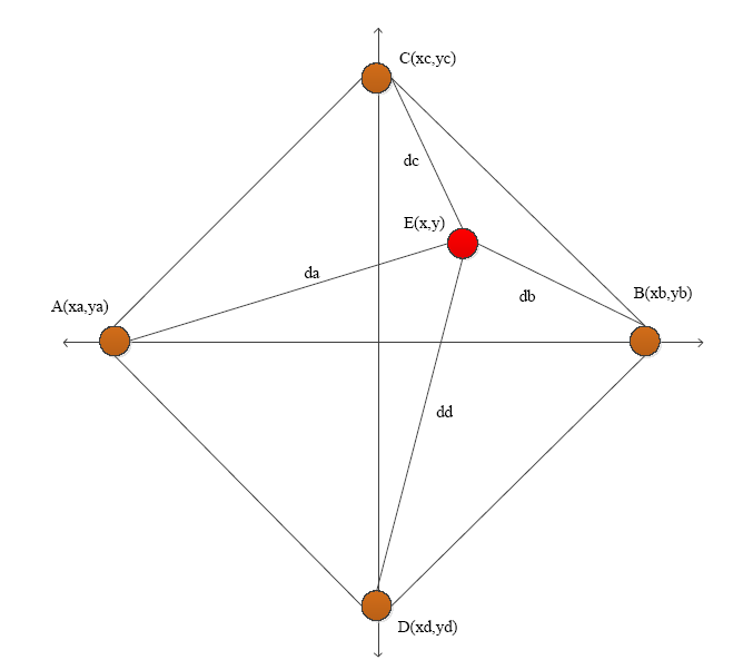
Figure 1.
Four-point AE localization planar geometry graph
According to the geometry relation between the AE source and AE sensors, the following equations exist:
In order to eliminate the quadratic term, the least squares method is used to solve Equation (1). Taking the first three equations successively to subtract the last one, a linear equation can be obtained as in Equation(2):
Where
$A=2\times \left[ \begin{matrix} {{x}_{a}}-{{x}_{d}} & {{y}_{a}}-{{y}_{d}} \\ {{x}_{b}}-{{x}_{d}} & {{y}_{b}}-{{y}_{d}} \\ {{x}_{c}}-{{x}_{d}} & {{y}_{c}}-{{y}_{d}} \\ \end{matrix} \right]$,$X=\left[ \begin{matrix} x \\ y \\\end{matrix} \right]$,$B=\left[ \begin{matrix} {{x}_{a}}^{2}-{{x}_{d}}^{2}+{{y}_{a}}^{2}-{{y}_{d}}^{2}+{{d}_{d}}^{2}-{{d}_{a}}^{2} \\ {{x}_{b}}^{2}-{{x}_{d}}^{2}+{{y}_{b}}^{2}-{{y}_{d}}^{2}+{{d}_{d}}^{2}-{{d}_{b}}^{2} \\ {{x}_{c}}^{2}-{{x}_{d}}^{2}+{{y}_{c}}^{2}-{{y}_{d}}^{2}+{{d}_{d}}^{2}-{{d}_{c}}^{2} \\\end{matrix} \right]$
The solution of Equation(2) is as follows:
According to the arrival time of the AE signals, the distance ${{d}_{i}}$(i =A, B, C, D) from the source to each sensor is calculated. By solving Equation(3), the location of the source (x, y) can be roughly calculated. Because of the subtraction process, some useful coordinate information of the AE sensors will be lost to yield large errors. In the meantime, the estimation of distance di is greatly affected by the accuracy of arrival time, which depends on the network induced delay. Therefore, a delay-weighted Taylor expansion algorithm is proposed in the following part to improve the localization accuracy.
2.2. Taylor Expansion Least Squares
In order to avoid the loss of accuracy by the subtraction process, the quadratic equation is linearized using the Taylor expansion formula.
Define the distance ${{d}_{i}}$ as follows:
f(x,y) is a Taylor expansion at the point (x0,y0):
By eliminating the remaining items ofEquation(5), Equation(1) can be deduced as
The initial value of (${{x}_{0}},{{y}_{0}}$) is calculated by Equation(3). The fault coordinate will be observed usingthe least squares method with the aim of satisfying the following Equation:
where ${{\varepsilon }_{threshold}}$ is the threshold, which depends on the maximum allowable localization error of x and y.If Equation(7) holds, the value of $({{x}_{0}},{{y}_{0}})$ is set as the coordinate of the source; otherwise, the next cycle is iterated. Let ${{x}_{1}}={{x}_{0}}+h,\text{ }{{y}_{1}}={{y}_{0}}+k$, and repeat this process until Equation(7) is satisfied. After the mth iteration, the coordinate (xm, ym) is set as the source coordinate.
3. Taylor’s Weighted Least Squares
3.1. Least Squares Weight Calculation Method
To improve the accuracy of the aforementioned Taylor expansion least squares estimation, the decomposed Equation(6) is weighted with the purpose of measuring the credibility of the data detected by AE sensors.
The original $AX=B$ is replaced by $WAX=WB$, where W is a weighted diagonal matrix as follows:
Equation(6) can be furtherrewrittenas
The solution of the weighted least squares method can be expressed as
3.2. Weighting Function Design
Considering the sensitivity of the positioning algorithm to network-induced delays, a weighting function is established to consider network-induced delays. Network-induced delays refer to the total duration from the detection time of AE sensors to the receiving time of the host. They include transmission delays, queuing delays, propagation delays, and processing delays. As mentioned in the first part, it is known that queuing delays, which are considered in the following, make up the majority of network induced delays. The wireless acoustic emission positioning system in the form of star topology is shown inFigure 2:
Figure 2.
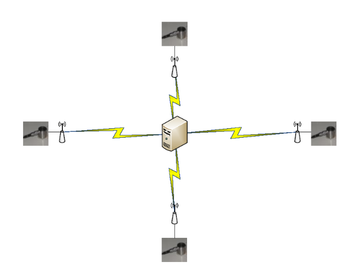
Figure 2.
AE network topology graph
Since the communication medium is shared, the AE sensors A, B, C, and D transmit the detected data to the host one by one. This requires that the transmission can only be executed under a priority. Non-preemptive priority, that is, when low-priority data is forwarded and high-priority data arrives, must wait until low-priority data is sent before forwarding the high-priority data [9]. Assume that the data in sensor i(i=A, B, C, and D) is divided into sdata packets and sent to the acoustic emission host in unit time. Suppose that the transmission time of each packet is ${{T}_{ik}}(k=1, 2, 3,\cdots , s)$ and the transmission rate is v. The sending rate of each sensor is the same, and thusv is constant. The average value of each packet’s transmission time is calculated by Equation(11).
Suppose that each acoustic emission sensor has sdata packets with priorities from lowto high for sensors A, B, C, and D, in unit time, respectively. The average transmission time ${{T}_{ik}}$ for each sensor is shown inFigure 3.
Figure 3.
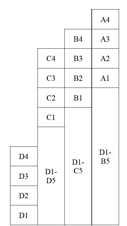
Figure 3.
Transmission time of each packet
InFigure 3, Di(i=1, 2, 3, 4, 5) represents the transmission delay of the ith packet of sensor D, Ci(i=1, 2, 3, 4, 5) represents the transmission delay of the ithpacket of sensor C, Bi(i=1, 2, 3, 4, 5) represents the transmission delay of the ith packet of sensor B, and Ai(i=1, 2, 3, 4, 5) represents the transmission delay of the ithpacket of sensor A.
As shown in Section 1, we consider the queuing delay as the transmission delay for this wireless network with star topology. Since the transmission medium air is shared by all the nodes of this network, the packet of each AE sensor has to wait for transmission until that the channel is free with the guidance of the priority scheme. As in Equation(11), the transmission time of sensor D means that the queuing time until the last packet is able to be transmitted. For sensor C with lower priority, its transmission time includes two parts, the transmission of s packets of sensor D and the transmission time of the first four packets of sensor C. This is formulated in Equation(12). The transmission times of sensorsA and B follow the same principle as sensor C, which is shown in Equations(13) and (14).
The average waiting time of sensor D is
The average wait time of sensor C is
The average waiting time of sensor B is
The average waiting time of sensor A is
Where ${{\eta }_{k}}=\frac{{{\alpha }_{ik}}}{v}$ is the waiting intensity and ${{\alpha }_{ik}}$ is the number of packets to be sent in unit time for the ithsensor.
The total occupation time of the medium for the ithsensor is the average waiting of this sensor ${{T}_{si}}$ plus the transmission time of one packet $\overline{{{T}_{ik}}}$, that is,
The delay induced weighting factor is defined as follows:
4. Experiment Analysis
In order to verify the effectiveness of the proposed weighted least squares localization algorithm in this paper, a simulation experiment is conducted.By taking a lead-break signal to simulate an AE source signal, all the data are detected by R3α AE sensors, preamp, and PCI-2 acquisition card (such as Figure 4) of Physical Acoustic Corporation (PAC). The resonant frequency is 90kHz, and the operating frequency range is 1 ~ 100kHz. The AE threshold is set to 40dB, and the sampling frequency is 4MHz. The lead breaking experiment is executed on a square iron plate with a width of 500mm. Four AE sensors are arranged as shown in Figure 5 in the experiment, and the coordinates are defined as A(-250, 0), B(250, 0), C(0, 250), and D(0,-250) with the unit of mm.
Figure 4.
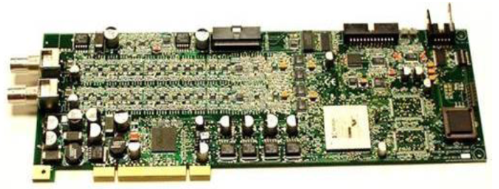
Figure 4.
PCI-2 acquisition card
Figure 5.
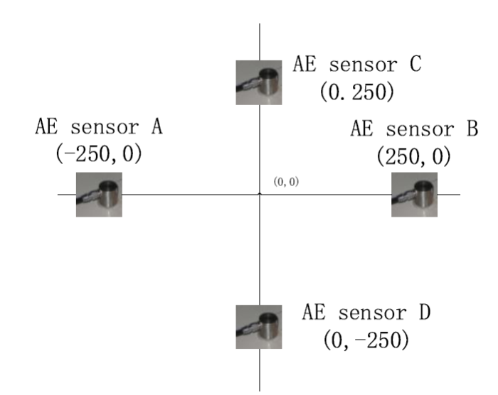
Figure 5.
AE sensors arrangement graph
PAC’s acoustic emission sensors are available in a variety of models from sensor size, center frequency, and interface form. The $R3\alpha $sensor has a size of 19mm×22mm, and the center frequency is 30kHz.
PCI-2has an 18-bit A/D, and the frequency range is 1 ~ 3kHz. It is able to store detection data into the hard disk continuously witha speed of 10Mbps.
AE sensors A, B, C, and D have priorities from low to high. With the data sampling time of 0.25 ms for each sensor, the data size is up to 336 M bps. According to the network protocol, the data is divided into five packets to transmit. The transmission rate v is 6 units/$\text{ }\!\!\mu\!\!\text{ s}$, and the transmission time $\overline{{{T}_{ik}}}$ is 0.17$\text{ }\!\!\mu\!\!\text{ s}$/units. The queuing parameters for the four sensors are shown in Figure 6.
Figure 6.
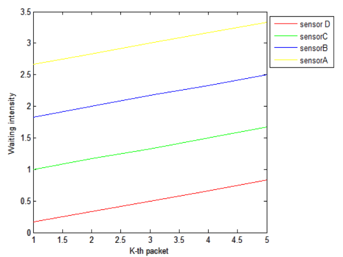
Figure 6.
The queuing parameters for the four sensors
Table 1. Waiting intensity of the ith sensor and kth packet
| i k | Sensor A | Sensor B | Sensor C | Sensor D |
|---|---|---|---|---|
| 1 | 2.67 | 1.83 | 1 | 0.17 |
| 2 | 2.83 | 2 | 1.17 | 0.33 |
| 3 | 3 | 2.17 | 1.33 | 0.5 |
| 4 | 3.17 | 2.33 | 1.5 | 0.66 |
| 5 | 3.33 | 2.5 | 1.67 | 0.83 |
The delays of the four sensors according to Equations (10) to (15) are shown in Table 2.
Table 2. Calculation results of each sensor’s delay
| Sensor | Ti | Hi |
|---|---|---|
| Sensor A | 5.294 | 5.464 |
| Sensor B | 2.885 | 3.055 |
| Sensor C | 1.185 | 1.355 |
| Sensor D | 0.197 | 0.367 |
According to the average queuing delay of each sensor, the weighting matrix W is expressed as
The maximum allowable errors of x and y are set as 20mm. The proposed localization algorithm is simulated in MATLAB software. The experiments are carried out with the lead-break signals at the coordinates of (0, 0), (10, 0), and (60, 0) withthe unit of mm. Compare the weighted positioning algorithm with the unweighted oneusing the following formula:
Where $\Delta x$ and $\Delta y$ are the error of coordinates between the calculated point and the lead-break point. The results are shown inFigure 7.
Figure 7.
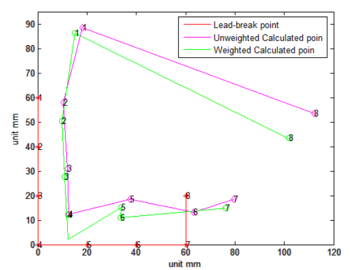
Figure 7.
Comparison of weighted and unweighted positioning algorithms
The absolute error and relative error are shown in Table 3.
Table 3. Comparison results of weighted and unweighted algorithms
| Positioning method | Lead-break point | Calculated point | Absolute error | Relative error |
|---|---|---|---|---|
| Weighted positioning algorithm | (0, 60) | (15.1, 86.2) | (15.1, 26.2) | 6.1% |
| (0, 40) | (9.8, 50.5) | (9.8, 10.5) | 2.9% | |
| (0, 20) | (10.8, 27.7) | (10.8, 7.7) | 2.7% | |
| (0, 0) | (12.4, 12.2) | (12.4, 12.2) | 3.5% | |
| (20, 0) | (33.9, 15.1) | (13.9, 15.1) | 4.1% | |
| (40, 0) | (33.7, 10.9) | (6.3, 10.9) | 2.6% | |
| (60, 0) | (76.1, 14.9) | (16.1, 14.9) | 4.4% | |
| (60, 20) | (101.8, 43.3) | (41.8, 23.3) | 9.6% | |
| Positioning method | Lead-break point | Calculated point | Absolute error | Relative error |
| Unweighted positioning algorithm | (0, 60) | (18.1, 88.6) | (18.1, 28.6) | 6.8% |
| (0, 40) | (10.5, 57.9) | (10.5, 17.9) | 4.2% | |
| (0, 20) | (11.9, 30.9) | (11.9, 10.9) | 3.2% | |
| (0, 0) | (12.5, 12.5) | (12.5, 12.5) | 3.5% | |
| (20, 0) | (37.4, 18.6) | (17.4, 18.6) | 5.1% | |
| (40, 0) | (63.2, 13.1) | (23.2, 13.1) | 5.3% | |
| (60, 0) | (79.6, 18.5) | (19.6, 18.5) | 5.4% | |
| (60, 20) | (112, 53.5) | (52, 13.5) | 10.7% |
As seen from Table 3, the accuracy of the weighted positioning algorithm is higher than that of the unweighted positioning algorithm. There are two main sources in the error analysis:
$\cdot$ Placement error of the acoustic emission sensors, which may affect the positioning accuracy greatly in the case of short-distance AE detection.
$\cdot$ Coordinate error of the stimulated source. The coordinate of lead break as a stimulated source is carried out by hand to influence the accuracy.
5. Conclusions
Acoustic emissionis one of the most widely used non-destructive testing techniques, and its high positioning accuracy has received extensive attention in the field.Based on the least squares method, the reliability of each AE sensor and the corresponding data are weighted concerning the network induced delay, and experiments are executed to verify the proposed algorithm.The results show that the modified algorithm with weighting factors can effectively improve the accuracy of AE localization.
In the future, other factors of network delay with different network protocols and topologies will be considered, and the deep research of wireless transmission delay mechanisms will also be investigated.
Acknowledgements
This work is supported by the School Fund of IMUT: Reliability Study of Wireless Networked Control System(ZD201503) and the Fault Diagnosis Research of the Networked Control System of High-Speed Train(NJZZ16085).
Reference
“Maximum Likelihood Network Localization using Range Estimation and GPS Measurements,
in
“Analysis of Queuing Delay and Medium Access Distribution over Wireless Multihop PANs,
”
“AUV Underwater Terrain Matching Location Method based on Maximum Likelihood Estimation,
“High Deadline Meeting Rate of Non-Preemptive Dynamic Soft Real Time Scheduling Algorithm,
in
DOI:10.1109/ICCSCE.2012.6487159
URL
[Cited within: 2]

Hard real time systems were often implemented with preemptive scheduling, which gives priority to the highest priority task. In this paper we present a new non-preemptive scheduling of jobs meant for soft real time application. Our ultimate aim is to increase the deadline meeting rate of the Earliest Deadline First (EDF) algorithm during overload condition while maintaining the optimum performance it poses during normal load. Our approach, grouped jobs with near deadlines together using our novel algorithm and schedule the jobs within a group using another algorithm. We named the approach Group, Utilization and Deadline Tolerance EDF (gutEDF). We will present result comparing the deadline meeting rate and average response time of gutEDF and EDF under different deadline tolerance values and compare the deadline meeting ratio improvement of gutEDF and gEDF.
“Exact Analysis of Weighted Centroid Localization, ”
in
“Dynamic Control Method of Queuing Delay with/without OEO Conversion in a Multi-Stage Access Network, ”
inTo respond to the diverse requirements of user and services, various technologies have been researched for future access networks. In particular, the optical access system should support wider dynamic range in bandwidth and various quality of service (QoS) metrics like latency. To realize these needs, a hybrid architecture node with optical and electrical layers is very attractive. It has the advantage of enhancing the delay performance by handling traffic in the optical layer without optical-electrical -optical (OEO) conversion. As one such approach, we have been studying a multi-stage access network with/without OEO conversion based on semiconductor optical amplifiers (SOAs); it makes it easy to provide the delay performance that each service requires. In this paper, we propose a method for controlling the number of OEO conversions; it uses a token bucket technique to realize the desired queuing delay performance. With this technique, the number of OEO conversions can be dynamically and freely controlled regardless of the traffic condition.
“Reproducible Data Processing Research for The CABRI R.I.A. Experiments Acoustic Emission Signal Analysis, ”
in
“An Improved APIT Location Algorithm for Wireless Sensor Networks, ”
DOI:10.1007/978-3-642-27951-5_17
URL
[Cited within: 1]
In order to improve localization accuracy and coverage of the APIT technique, we proposed an improved localization algorithm which further employed the RSSI range method with the APIT technique. Namely, we performed an extra RSSI value comparison in carrying out Point-In-Triangulation test to reduce the Out-To-In errors. Furthermore, we used intersection of two anchor circles to solve the problem when the number of nearby anchor nodes was insufficient for localization. Simulation results show that using the proposed algorithm, localization accuracy can be increased by about 11% when the density of nodes is relatively low. Meanwhile, the proposed algorithm can achieve better coverage comparing with the classic APIT algorithm.
“AFCD: An Approximated-Fair and Controlled-Delay Queuing for High Speed Networks, ”
in
DOI:10.1109/ICCCN.2013.6614103
URL
[Cited within: 1]
High speed networks have characteristics of high bandwidth, long queuing delay, and high burstiness which make it difficult to address issues such as fairness, low queuing delay and high link utilization. Current high speed networks carry heterogeneous TCP flows which makes it even more challenging to address these issues. Since sender centric approaches do not meet these challenges, there have been several proposals to address them at router level via queue management (QM) schemes. These QM schemes have been fairly successful in addressing either fairness issues or large queuing delay but not both at the same time. We propose a new QM scheme called Approximated-Fair and Controlled-Delay (AFCD) queuing for high speed networks that aims to meet following design goals: approximated fairness, controlled low queuing delay, high link utilization and simple implementation. The design of AFCD utilizes a novel synergistic approach by forming an alliance between approximated fair queuing and controlled delay queuing. It uses very small amount of state information in sending rate estimation of flows and makes drop decision based on a target delay of individual flow. Through experimental evaluation in a 10Gbps high speed networking environment, we show AFCD meets our design goals by maintaining approximated fair share of bandwidth among flows and ensuring a controlled very low queuing delay with a comparable link utilization.
“Centroid Location Algorithm for Wireless Sensor Networks based on Optimal Beacon Nodes, ”
“Using the Steepest Descent Algorithm to Improve the Node Location Accuracy of the Maximum Likelihood Estimation Algorithm, ”
“Generalized Cross Correlation Time Delay Estimation Sound Localization Algorithm, ”
“Analysis of Time Delay in Networked Control Systems and Study of Data Transmission Technology, ”
“Quadratic Correlation Time Delay Estimation Algorithm based on Kaiser Window and Hilbert Transform, ”
in
DOI:10.1109/IMCCC.2016.149
URL
[Cited within: 1]
There is a tiny difference between the main peak and side peaks after the traditional quadratic correlation calculation in the time-delay estimation of passive acoustic positioning system. It is easy to lead to a wrong peak value when the system resolution is low or mutations caused by noises occur near the side peaks. In order to weaken the influence of the quadratic correlation side peaks, the method of using the characteristic of the Kaiser window to improve the weighting way is proposed. Using Hilbert transform to sharpen the correlation peak can make up the drawback of correlation peak widened by the Kaiser window. The experimental simulation results show that this method can effectively enhance anti-noise ability of time-delay estimation.
“Two-Stage Centroid Localization for Wireless Sensor Networks using Received Signal Strength, ”
inA two-stage centroid localization algorithm for wireless networks (WSNs) based on received signal strength (RSS) is proposed. In the first stage, the unknown node performs symmetric lens presence tests to construct a virtual neighboring anchor list. By using the locations of two neighboring anchors and the RSS relationships, a symmetric lens presence test determines a residence area of the unknown node which is geometrically shaped as a half-symmetric lens. The centroid of the estimated residence area is then defined as a virtual neighboring anchor. In the second stage, the location of the unknown node is estimated based on the virtual neighboring anchor locations, using the centroid formula. Simulation results show that the proposed method has better performance compared to other two typical range-free localization methods.
“Channel-based Sampling Rate and Queuing State Control in Delay-Constraint Industrial WSNs , ”
in
DOI:10.1109/GLOCOM.2017.8253933
URL
[Cited within: 1]
Industrial Wireless Sensor Networks (IWSNs) improve the transmission precision of control signaling as well as contributing to the real-time data monitoring and instrument fault diagnosing throughout the manufacturing production. However, wireless channel effects, such as multipath attenuations, noise and co- channel interference, may have unpredictable and time-varying impacts on keeping packets transmission delay. To address this issue, we propose a Channel-based Sampling rate and Queuing state Control (CSQC) scheme to minimize the packet transmission delay in IWSNs. Specifically, we explore the rapid fading characteristics of the industrial wireless channel by studying the level crossing rate (LCR). We develop a continuous-time Markov model to evaluate the packet sojourn time and design an expectation-maximization (EM) algorithm to timely calibrate the transition rate in the model. Finally, we optimize the sensor sampling rate and queuing state to minimize the packet queuing delay in IWSNs. Simulation results show that the CSQC scheme has lower delay than IEEE 802.15.4 standard does under varying interference effects.
“A Linear Least Square Method for Sound Source Target Precise Localization, ”
“ComLoB: Link Quality and Queuing Delay based Composite Routing Protocol for Traffic Load Balancing in WSNs, ”
in
“A Novel DV-Hop Method for Localization of Network Nodes, ”
in
DOI:10.1109/ChiCC.2016.7554686
URL
[Cited within: 1]
According to the characteristics of WSN with mass nodes, a DV-Hop localization method improved by the shuffled frog leaping algorithm (SFLA) for WSNs was proposed in this paper. Considering the shortages of the traditional DV-hop localization algorithm, the calculation of average hop distance is improved, and the average hop distance can be calculated by SFLA, which can reduce the error of distance estimation for average hop and improve the localization accuracy of the algorithm. In addition, the localization error of unknown nodes is further reduced by the optimization process of nodes swap. The simulation results indicate that the improved DV-Hop algorithm can reduce the localization error and the degree of dependency for beacon nodes and network connectivity effectively.
“DV-HOP Triple Localization Algorithm, ”
“Based on The Cyclic Refinement APIT Localization Algorithm for Wireless Sensor Networks, ”
in
“Study of Positioning of Rock Acoustic Emission Source based on Phase Difference Time Delay Estimation, ”
“DV-HOP Localization Algorithm with Weight-based Oriented Cuckoo Search Algorithm, ”
in
DOI:10.23919/ChiCC.2017.8027742
URL
[Cited within: 1]
Oriented cuckoo search algorithm(OCS) is a newly proposed variant of cuckoo search algorithm, to avoid the premature convergence, weighted-based oriented cuckoo search(WOCS) is proposed which is a combination of OCS and the standard CS.WOCS achieves a balance between exploration and exploitation.To test the performance, WOCS is incorporated into the methodology of DV-Hop localization algorithm for node localization in wireless sensor networks.The simulation results show that DV-Hop localization with WOCS achieves best positioning accuracy when compared with other two algorithms.
“Localization in Sensor Networks with Communication Delays and Package Losses, ”
in
“A Price-based Interactive Data Queue Management Approach for Delay-Tolerant Mobile Sensor Networks, ”
in
DOI:10.1109/WCNCW.2013.6533338
URL
[Cited within: 1]
This paper presents a price-based interactive data queue management approach (PI-DQM) for delay-tolerant mobile sensor networks (DT-MSNs) to address the priority deviation problem during the data transmission process. Three interactive parameters are introduced and weighted values 伪 and the p-value are used in the price-based interaction model to identify the data priority. The method is transparent to prioritized data packets. Its effectiveness is illustrated by showing that it can ameliorate the data delivery ratio and achieve good performance in terms of average delay.
“SDLSne - Improved Scalable Distributed Least Squares Localization with Minimized Communication, ”
in
DOI:10.1109/PIMRC.2010.5671924
URL
[Cited within: 1]
Wireless Sensor Networks (WSNs) have been of high interest during the past couple of years. One of the most important aspects of WSN research is location estimation. As a good solution of fine grained localization Reichenbach et al. introduced the Distributed Least Squares (DLS) algorithm, which splits the costly localization process in a complex precalculation and a simple postcalculation which is performed on constrained sensor nodes to finalize the localization by adding local knowledge. This approach lacks for large WSNs, because cost of communication and computation theoretically increases with the network size. In practice the approach is even unusable for large WSNs. This restriction have been overcome by scalable DLS (sDLS), which enabled to use the idea of DLS in large WSNs for the first time. Although, sDLS outperforms DLS for large networks, cost of communication and computation is initially higher for small networks, caused by data updates. The approach, presented in this work, dramatically reduces cost of communication of sDLS. Additionally, a new approach of distance estimation is applied to original DLS. In contrast to earlier simulations, this leads to improved localization, which is used for fairer comparison.
“Online Particle Size Measurement Through Acoustic Emission Detection and Signal Analysis, ”
in
“Improved APIT Localization Algorithm in Wireless Sensor Networks, ”
in
“A Bluetooth Location Method based on Least Squares, ”
“Delay Analysis of Max-Weight Queue Algorithm for Time-Varying Wireless Ad hoc Networks—Control Theoretical Approach, ”
“Computer Networks Stability Independence of the Queuing Delays, ”
in
“Performance Analysis of Throughput and Queuing Delay for Multiple Optical Channels for Local Area Network, ”
in
DOI:10.1109/ISMS.2014.44
URL
[Cited within: 1]
The advances in Wavelength Division Multiplexing (WDM) technology have tremendously increased the bandwidth of a single fiber optic, for local and metropolitan area network (LAN and MAN). This paper presents and discusses a new network environment that is multiple optical channel, which coupled Ethernet with WDM to decrease the average queuing delay and increases the normalized throughput. The performances of three channels are evaluated with different network parameters using discrete event simulator called OMNeT++. In this paper it has been proved that RS BEB algorithms show the best throughput for three data rates. Moreover, in average queuing delay and RS BEB shows the lowest delay despite the others algorithms. It has been observed from this work that an increase in the number of nodes, the percentage of normalized throughput decreasing is less than 20% for every additional node in the network.
“Novel Passive Localization Algorithm based on Double Side Matrix-Restricted Total Least Squares, ”
DOI:10.1016/j.cja.2013.06.009
URL
[Cited within: 1]
In order to solve the bearings-only passive localization problem in the presence of erroneous observer position, a novel algorithm based on double side matrix-restricted total least squares (DSMRTLS) is proposed. First, the aforementioned passive localization problem is transferred to the DSMRTLS problem by deriving a multiplicative structure for both the observation matrix and the observation vector. Second, the corresponding optimization problem of the DSMRTLS problem without constraint is derived, which can be approximated as the generalized Rayleigh quotient minimization problem. Then, the localization solution which is globally optimal and asymptotically unbiased can be got by generalized eigenvalue decomposition. Simulation results verify the rationality of the approximation and the good performance of the proposed algorithm compared with several typical algorithms.
“Locating The Position of Objects in Non-Line-of-Sight based on Time Delay Estimation, ”
DOI:10.1088/1674-1056/25/8/084203
URL
[Cited within: 1]
Non-line-of-sight imaging detection is to detect hidden objects by indirect light and intermediary surface(diffuser).It has very important significance in indirect access to an object or dangerous object detection, such as medical treatment and rescue. An approach to locating the positions of hidden objects is proposed based on time delay estimation. The time delays between the received signals and the source signal can be obtained by correlation analysis, and then the positions of hidden objects will be located. Compared with earlier systems and methods, the proposed approach has some modifications and provides significant improvements, such as quick data acquisition, simple system structure and low cost, and can locate the positions of hidden objects as well: this technology lays a good foundation for developing a practical system that can be used in real applications.
