Fatigue Life Prediction for Throwing Impeller of an Impeller Blower

doi:10.23940/ijpe.19.01.p13.127137

Fatigue Life Prediction for Throwing Impeller of an Impeller Blower

Zhiping Zhai^a, Can Li^a, Hongmei Cui^,^b, Hongyu Liang^a, and Haiying Cheng^a

a College of Mechanical Engineering, Inner Mongolia University of Technology, Hohhot, 010051, China

b College of Mechanical and Electrical Engineering, Inner Mongolia Agricultural University, Hohhot, 010018, China

Corresponding authors: * E-mail address: chm123m@126.com

Accepted: 2018-12-17 Online: 2019-01-1

Abstract

Impeller blowers are used to convey materials for various forage harvesters. As the main working component, the throwing impeller endures various static and dynamic loads while conveying the materials. This makes the throwing impeller prone to fatigue fracture, so it is very necessary to find a feasible model to estimate the fatigue life of the throwing impeller accurately. In order to obtain the accurate random cyclic load applied on the high-speed rotating impeller, the finite element analysis and the fluid-solid coupling method are adopted to calculate the stress distribution of the impeller under the combined action of the fluid-solid coupling flow field pressure, the centrifugal force, and the gravity. At the same time, the stress on the dangerous section of the impeller is measured by using the DH5909 wireless strain testing system and is compared with the calculated one. The contrast results show that the numerical calculation results are reliable. To accurately predict the fatigue life of the throwing impeller at the design stage, the two-parameter nominal stress model is deduced and combined with the linear cumulative damage model of Miner and the log normal distribution model. Its two parameters of the average stress S_m and the stress amplitude S_a can be obtained through finite element analysis and do not have to be equivalent to a symmetrical cyclic load. Therefore, its precision of estimating the fatigue life is improved. By contrasting the rated and predicted fatigue lives of an impeller, it was found that the impeller’s actual rated lives are closer to the predicted lives of the Goodman and Gerber two-parameter nominal stress model than those of the conventional S-N curve. In particular, they are closer to the calculation results of the Gerber-type two-parameter nominal stress model. This shows that the Gerber-type two-parameter nominal stress model is more accurate and suitable to predict the fatigue life of the throwing impeller. These achievements will play a significant role in further optimizing the impeller and improving its reliability.

Keywords: throwing impeller; fatigue life; two-parameter nominal stress model; Miner rule; log-normal distribution

PDF (788KB) Metadata Related articles Export EndNote| Ris| Bibtex Favorite

Cite this article

Zhiping Zhai, Can Li, Hongmei Cui, Hongyu Liang, and Haiying Cheng. Fatigue Life Prediction for Throwing Impeller of an Impeller Blower. International Journal of Performability Engineering, 2019, 15(1): 127-137 doi:10.23940/ijpe.19.01.p13.127137

List of Symbols

MMaterial constant

CMaterial constant

N Fatigue life

S_max Maximum alternating stress

S_m Average stress

S_a Stress amplitude

R Stress ratio

S_-1 Fatigue limit of material under the actionof symmetric cyclic load

S_bUltimate strength of material

K_S Effective stress concentration factor

ε_S Size factor

β Surface quality coefficient

φ_S Sensitivity coefficient of material to the asymmetry of cycle stress

n Actual cyclic number

D Damage fraction

k Stress levels number

n_i Actual cyclic number there are k different stress levels in one cycle

S_aiAverage stress at aconstant amplitude stress level

S_miStress amplitude at aconstant amplitude stress level

N_i Average number of cycles to failureat a constantamplitude stress level (S_ai, S_mi)

x Random variable of fatigue life

μ Logarithmic mean deviation

σ Logarithmic standard deviation

E(X) Mean deviation

$\sqrt{D(X)}$ Standard deviation

$\Phi \left( \frac{\ln x-\mu }{\sigma } \right)$ Standard normal distribution function

1. Introduction

An impeller blower generally consists of the throwing impeller, shell, and discharge tube. This device is widely used to convey materials in various forage harvesters because of its simplicity, reliability, easy maintenance, high capacity, and low manufacturing cost [1]. As the core working component, the throwing impeller often endures the combined action of the centrifugal force, the gravity, and the varying pressure of high-speed air flow and materials inside the impeller blower. This will accelerate the throwing impeller’s fatigue, leading to fracture [2]. In recent years, most research on impeller blowers mainly focused on reducing the power consumption as well as increasing the throwing distanceand efficiency [3-6]. However, relatively few data exist on the topic of investigating the fatigue life of the throwing impeller. Thus, it is very necessary to find a feasible model to accurately estimate the fatigue life of throwing impellers.

Research works on the fatigue life for the similar rotating machine are presented as follows.Dileep [7] estimated the low-cycle fatigue life of a centrifugal impeller under the engine operating conditions by using four different multi-axial fatigue damage models. The predicted lives were then compared with the experimental value obtained from the cyclic spin test. The critical plane-based models showed better prediction accuracy and capability in comparison to the maximum von Mises strain range model. Shanmugam[8] estimated the fatigue life of a titanium alloy centrifugal impeller by using the equivalent strain method and Smith Watson Topper (SWT) method and assessed the fatigue life via the cyclic spin test. The probabilistic analysis of fatigue life was carried out by using the Weibull distribution method. It was found that the equivalent strain method is nonconservative due to the exclusion of the mean stress effect. The average fatigue life of the impeller was estimated at 12000 cycles by using the SWT method, which was closer to the test results. Xu[9] analyzed the fatigue life of a remanufactured centrifugal compressor impellers by using the S-N curve data and the rain-flow counting method based on FEA. It was found that the simulation results were useful for analyzing fatigue life impact factors and fatigue fracture areas, although it was incapable of providing high-precision prediction. Liao and Huang[10] investigated the fatigue life of a turbine disk by constructing Goodman and Gerber types of a generalized σ-N curved surface equation based on stress amplitude and mean stress. An aircraft engine turbine disk was presented to validate the proposed method. The results showed that the prediction of the Goodman equivalent life curve was much more accurate than that of the Gerber type model. This method also showed better accuracy for estimating the fatigue life than the conventional S-N curve. Pavlou [11] presented a new theory for macroscopic fatigue damage estimation based on the S-N curve, which was a generalization of most of the existing fatigue damage models. Saggar [12] presented a fatigue damage cumulative model under the variable load devoted for defective materials. This model was connected cycle by cycle with the S-N curve, and it also took into account the loading history. The predicted results of this model were compared with the experimental results for a C35 low alloy steel containing defects and those computed by Miner’s model. It was demonstrated that the proposed model predicted the fatigue damage much better than the Miner rule.

From the research above, in order to ensure safe and reliable operation of the throwing impeller, the two-parameter (namely the average stress S_m and the stress amplitude S_a) nominal stress model, the cumulative damage model of Miner, and the logarithm normal distribution model are combined to estimate the fatigue life of the impeller in this paper. In addition, the fluid-solid coupling method in the finite element analysis is used to accurately obtain the random cyclic dynamic stress distribution of the throwing impeller under the combined effect of the flow field pressure, centrifugal force, and gravity. The stress on the dangerous cross section of the impeller at the empty load is also tested by using the DH5909 wireless strain test system. Then, the measured stresses are compared with the simulated ones via the finite element numerical calculation. After verifying the correctness of the numerical model, the fatigue life of a throwing impeller under the working load will be predicted by calculating the variation of stress along with time at the maximum stress point of the impeller’s critical section.

The rest of this article is organized as follows. Section 2 proposes the fatigue reliability theory model for structures under the random cyclic load. Section 3 provides a numerical calculation method on the stress distribution of a high-speed rotating impeller. The fatigue life prediction of an impeller blower is presented in Section 4. Finally, Section 5presents three conclusions.

2.Theory of Fatigue Reliability

2.1.Two-Parameter Nominal Stress Model

According to the S-N curve and the constant life curve of material, the two-parameter nominal stress equation including the average stress S_m, the stress amplitude S_a, and the fatigue life N can be deduced as follows [12-13].

Considering that the throwing impeller belongs to the high cycle fatigue, the relationship between its maximum alternating stress S_max and the fatigue life of N is given by

(1) $S_{\max }^{m}N=C$

Where m and C are the material constants.

The relationship including the maximum alternating stress S_max, the average stress S_m, and the stress amplitude S_a can be expressed as follows:

(2) ${{S}_{\max }}=\frac{2{{S}_{m}}}{1+r}$

(3) ${{S}_{a}}=\left( \frac{1-r}{1+r} \right){{S}_{m}}$

Where r is the stress ratio.

Substituting Equation (2)into Equation (1),Equation (4)will be obtained as follows:

(4) ${{S}_{m}}=\frac{1+r}{2}{{\left( \frac{C}{N} \right)}^{1/m}}$

Substituting Equation (4)into Equation (3),S_a can be expressed as follows:

(5) ${{S}_{a}}=\frac{1-r}{2}{{\left( \frac{C}{N} \right)}^{1/m}}$

Because the impeller is running at the random cyclic load, the S-N curve that is more suitable for the condition of the symmetrical cyclicload needs to be revised. Thus, the Goodman formula is selected as the constant life curve, as follows:

(6) $\frac{{{S}_{a}}}{{{S}_{-1}}}+\frac{{{S}_{m}}}{{{S}_{b}}}=1$

WhereS_b is the ultimate strength of the material and S_-1 is the fatigue limit of the material under the actionof the symmetric cyclic load.

Substituting Equations (4) and (5) into Equation (6), Equation (7) can be obtained as follows:

(7)${{S}_{-1}}=\frac{{{S}_{b}}(1-r){{(C/N)}^{1/m}}}{2{{S}_{b}}-(1+r){{(C/N)}^{1/m}}}$

Substituting Equation(7) into Equation(6), the average stress S_m will be obtained as follows:

(8) ${{S}_{m}}=\frac{\left[ (1+r){{S}_{a}}+(1-r){{S}_{b}} \right]{{(C/N)}^{1/m}}-2{{S}_{a}}{{S}_{b}}}{(1-r){{(C/N)}^{1/m}}}$

Then, the two-parameter nominal stress equation of Goodman type is expressed as follows:

(9) ${{\left[ \frac{2{{S}_{a}}{{S}_{b}}}{(1+r){{S}_{a}}+(1-r)({{S}_{b}}-{{S}_{m}})} \right]}^{m}}N=C$

If we choose the Gerber formula as the constant lifecurve [14],

(10) ${{\left( \frac{{{S}_{m}}}{{{S}_{b}}} \right)}^{2}}+\left( \frac{{{S}_{a}}}{{{S}_{-1}}} \right)=1$

The two-parameter nominal stress equation of Gerber type can be similarly obtained as follows:

(11) ${{\left\{ \frac{{{\left[ {{\left( 1-r \right)}^{2}}{{\left( S_{b}^{2}-S_{m}^{2} \right)}^{2}}+4S_{a}^{2}{{\left( 1+r \right)}^{2}}S_{b}^{2} \right]}^{1/2}}-\left( 1-r \right)\left( S_{b}^{2}-S_{m}^{2} \right)}{{{S}_{a}}{{\left( 1+r \right)}^{2}}} \right\}}^{m}}N=C$

2.2.Two-Parameter Nominal Stress Model of a Throwing Impeller

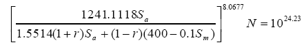
If we apply the S_a-S_m-N two-parameter nominal stress models of material into estimating the fatigue life of the actual throwing impellers, the factors including the stress concentration, size, surface quality, and sensitivity of impeller material to the asymmetrical cycle stress that affect the fatigue strength of the impeller must be considered[15]. The revised Goodman-type two-parameter nominal stress equation is listed as follows:

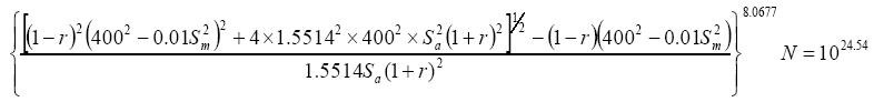
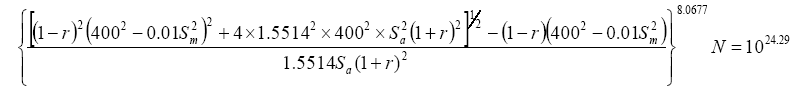
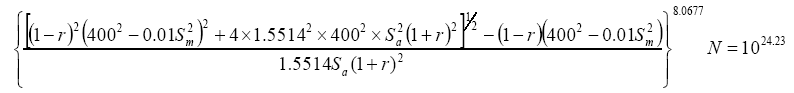
(12) ${{\left[ \frac{\left( 2\frac{{{K}_{S}}}{{{\varepsilon }_{S}}\beta } \right){{S}_{a}}{{S}_{b}}}{\left( 1+r \right)\left( \frac{{{K}_{S}}}{{{\varepsilon }_{S}}\beta } \right){{S}_{a}}+\left( 1-r \right)\left( {{S}_{b}}-{{\varphi }_{S}}{{S}_{m}} \right)} \right]}^{m}}N=C$

The revised Gerber-type two-parameter nominal stress equation is listed as follows:

(13) ${{\left\{ \frac{{{\left[ {{\left( 1-r \right)}^{2}}{{\left( S_{b}^{2}-\varphi _{S}^{2}S_{m}^{2} \right)}^{2}}+4{{\left( \frac{{{K}_{S}}}{{{\varepsilon }_{S}}\beta } \right)}^{2}}S_{a}^{2}{{\left( 1+r \right)}^{2}}S_{b}^{2} \right]}^{1/2}}-\left( 1-r \right)\left( S_{b}^{2}-\varphi _{S}^{2}S_{m}^{2} \right)}{\left( \frac{{{K}_{S}}}{{{\varepsilon }_{S}}\beta } \right){{S}_{a}}{{\left( 1+r \right)}^{2}}} \right\}}^{m}}N=C$

Where ${{K}_{S}}$ is the effective stress concentration factor of the impeller, ${{\varepsilon }_{S}}$ is the size factor, $\beta$ is the surface quality coefficient, and ${{\varphi }_{S}}$ is the sensitivity coefficient of the impeller material to the asymmetry of the cycle stress.

2.3. Miner Cumulative Fatigue Damage Model

The throwing impeller always works under the condition of the alternating loads with different frequencies and different amplitudes. Its fatigue damage will accumulate to a certain extent, leading to the impeller’s fracture. Thus, the average stress and stress amplitude should be considered forthe fatigue strength analysis. According to the two-parameter nominal stress Formula (12) and Formula (13), the fatigue damage of the impeller under the cyclic load at certain stress level (S_a, S_m) can be directly calculated.

Miner’s cumulative damage theory assumes that the damage is accumulated linearly. Each cycle will cause some damage to the material when the material is subjected to the higher stress than the fatigue limit. For some components under the actions of constant amplitude stress level (S_a, S_m), the fatigue damage caused by each cycle is 1/N(S_a, S_m). The fatigue damage caused by ncycles is calculated as follows:

(14) $D=\frac{n({{S}_{a}},{{S}_{m}})}{N({{S}_{a}},{{S}_{m}})}$

Where n is the actual cyclic number andN is the numberof cycles to failureat a particular stress level (S_a, S_m). Failure is expected to occur when n is equal to N or D is equal to one.

As far as the throwing impeller at different amplitude stress levels is concerned, its damage fraction D is expressed as follows under the condition that there are k different stress levels applied on the impeller in one cycle and the average number of cycles to failure after n_icycles at aconstant amplitude stress level of S_ai and S_mi is N_i. The fatigue damage caused by n_icycles is calculated as follows:

(15)$D=\sum\limits_{i=1}^{k}{{{D}_{i}}}=\sum\limits_{i=1}^{k}{\frac{{{n}_{i}}({{S}_{ai}},{{S}_{mi}})}{{{N}_{i}}({{S}_{ai}},{{S}_{mi}})}}$

When these damage add up to one, the impeller will experience fatigue failure.

In this way, there isonly one-to-one transformation between each fatigue damage andeach load cycle represented by the two-parameter amplitude and mean value. Because the equivalent transformation of stresses does not need to be carried out, the estimating accuracy of the fatigue life is improved.

2.4.Fatigue Life Lognormal Distribution Model

Due to the randomness of the basic variables such as load, material parameters, and geometrical parameters of the impeller in the working process, the fatigue life shows discreteness. The throwing impeller’s material is Q235, and its fatigue life distribution obeys the log normal distribution according to the existing research [16].

Under the action of the cyclic load, the distribution law of the impeller’s fatigue life can be expressed by the log normal probability density function [17]as follows:

(16) $\begin{matrix} & f(x)=\left\{ \begin{matrix} \frac{1}{x\sigma \sqrt{2\pi }}\exp \left[ -\frac{1}{2}{{\left( \frac{\ln x-\mu }{\sigma } \right)}^{2}} \right],\text{ }x>0,\text{ }\sigma >0,\text{ }-\infty <\mu <\infty \\ 0,\text{ }x\le 0 \\ \end{matrix} \right. \\ & \\ \end{matrix}$

Where x is a random variable of the fatigue life andμ and σ are the logarithmic mean and standard deviation respectively.

The distribution function of the log normal distribution is given by the following formula:

(17) $\begin{matrix} & F(x)=P\left\{ X\le x \right\}=\int_{0}^{x}{\frac{1}{x\sigma \sqrt{2\pi }}\exp \left[ -\frac{1}{2}{{\left( \frac{\ln x-\mu }{\sigma } \right)}^{2}} \right]\text{d}x} \\ & \\ \end{matrix}$

Mean E(X) and the standard deviation $\sqrt{D(X)}$ are calculated by using the following two formulas:

(18) $E(X)=\exp \left( \mu +\frac{{{\sigma }^{2}}}{2} \right)$

(19) $D(X)=\exp \left( 2\mu +{{\sigma }^{2}} \right)\left( \exp {{\sigma }^{2}}-1 \right)$

The reliability function of the log normal distribution is expressed as follows:

(20) $P(x)=1-F(x)=\int_{x}^{\infty }{\frac{1}{x\sigma \sqrt{2\pi }}\exp \left[ -\frac{1}{2}{{\left( \frac{\ln x-\mu }{\sigma } \right)}^{2}} \right]\text{d}x=1-\Phi \left( \frac{\ln x-\mu }{\sigma } \right)}$

Where $\Phi \left( \frac{\ln x-\mu }{\sigma } \right)$ is the standard normal distribution function.

3. Fluid-Structure Coupling and Stress Analysis of the Impeller

The flow field pressure distribution inside the impeller blower is very complex and difficult to be measured directly. In order to accurately get the flow field and load distribution onimpellers, the numerical calculation of the gas-solid two-phase flow in the impeller blower is carried out by using the FLUENT. The ANSYS Workbench is also used to carry out the fluid-solid-solid (air-material-impeller) coupling process. The pressure generated by the gas-solid flow field as well as the centrifugal force and gravity areloaded on the impeller. The stress distribution of the impeller is obtained. Then, the stress of the impeller under the unloaded condition is measured to verify thenumerical calculation results by using the DH5909 wireless strain test system. After that, the stress distribution of the throwing impeller under the loading condition is calculated by using the ANSYS Workbench.

3.1. Finite Element Model and Meshing of the Impeller

The three-dimensional modelling software Pro/E is used to build a three-dimensional solid model of the impeller. The three-dimensional solid model of the impeller is then imported into HyperMesh for meshing. The numbers of cells and nodes of the entire impeller model inthe finite element mesh are 26, 800 and 40, 532 respectively [18].

3.2. Fluid-Structure Coupling Analysis

The flow channel model of the impeller blower is established in Fluent at first. The large eddy simulation(LED) model is used to simulate the unsteady flow field in the impeller blower. The variation law of the instantaneous fluctuation pressure in the single-phase airflow field and the flow field pressure distribution on the impeller surface will be obtained.

Then, the Fluent and Workbench coupling analysis platform is used to exert the simulated flow field pressureas well as the centrifugal force and gravity to the coupling surface of the impeller. Constraints are also imposed on the impeller to restrict its reciprocating motions in theX, Y, and Z directions and rotational motions around the X and Z axes. There is only onedegree of freedom of theY-axis rotation left. The impeller’s speed is 1500r/min.

3.3. Stress Analysis of the Throwing Impeller

Under the combined action of the above loads, the equivalent stress of the impeller underthe unloaded state is calculated by using the finite element method as shown in Figure 1. By using the post-processing tools in the Workbench software, the maximum stress is detected, which is 25.435MPa at the junction of the blade root and the stiffener. This is due to the stress concentration caused by the sharp change of the geometric shape and the thickness at thejoint.

Figure 1.

New window| Download| PPT slide

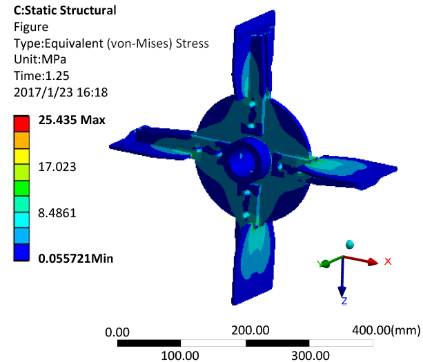
Figure 1. The equivalent stress cloud of the throwing impeller under the unloaded condition

Set the stress monitoring point in the area with the biggest stress as shown in Figure 2. Thestress simulation results in 0.25 seconds at the monitoring point are illustrated in Figure 3 when the impeller rotates at a speed of 1500r/min in the unloaded and stable condition.

Figure 2.

New window| Download| PPT slide

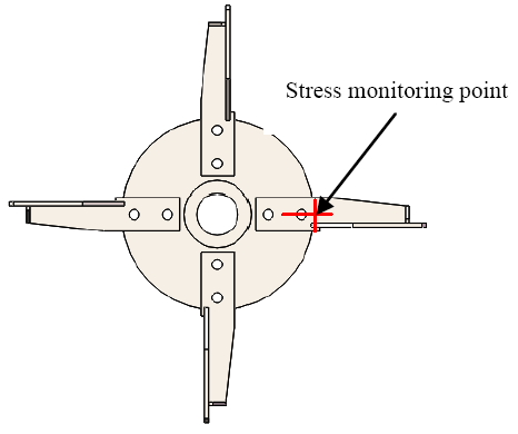
Figure 2. The measuring point distribution diagram of the impeller’s strain

Figure 3.

New window| Download| PPT slide

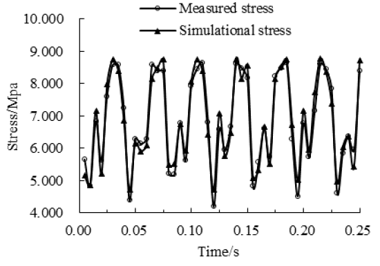
Figure 3. Comparisons between the measured and simulated stress of the impeller under the unloaded condition

It can be seen from Figure 3 that the dynamic loads at the monitoring point are changing according to the random cyclic and quasi-periodic variables, and the period of the stress variation is the same as the impeller rotation period. The maximum stress is 8.763MPa, the minimum is 4.721MPa, and the average stress is 6.880MPa.

3.3.1. Strain Test of the Throwing Impeller

In order to verify the correctness of the Finite Element calculation results, the DH5905 wireless strain tester developed by Tung Wah Testing Technologies Co., Ltd. is used to test the strain of the impeller. Considering that the test system would interfere with the throwing performance of materials under the loaded condition, the impeller’s stress is measured only for the unloaded condition. The test flow chart is shown in Figure 4.

Figure 4.

New window| Download| PPT slide

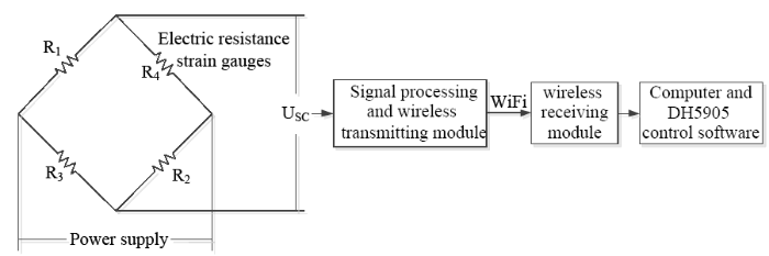
Figure 4. Strain test block diagram by using Dh5905 wireless strain gauge

An AC full-bridge circuit of Wheatstone bridge is formed to measure the impeller’s strain. The strain gauges are arranged on the impeller rotating at a high speed of 1500r/min(Figure 5). Because theimpeller’s strain signalsare not convenient for the wire transmission in the closed shell, the DH5905 wireless strain gauge test system is adopted. The entire test system, including four strain gauges, one power module, one signal conditioning and wireless transmitting module, one wireless receiving module, and DH5905 signal processing software, is shown in Figure 4. The strain of the impeller under the unloaded condition is measured by the strain gauge. Then, this weak strain signal is amplified and transmitted to the wireless receiving module by the Wheatstone Bridge and signal conditioning and wireless transmitting module. After passing through the WiFi wireless receiving module, the amplified real-time strain signal is stored on the computer and displayed dynamically on the interface of the DH5905 signal processing software.

Figure 5.

New window| Download| PPT slide

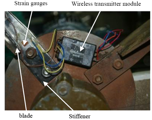
Figure 5. The connection diagram of strain gauges and wireless transmitting module

Because the maximum stress point is not suitable for pasting the strain gauge, an extension area of the two bolt hole axis of the stiffener near the maximum stress is chosen as the test point shown in Figure 5. For the accurate comparison, the simulated stress monitoring point is set as the same as this position shown in Figure 2. The maximum principal strain direction of the strain gauge is the same as that of the centrifugal force of the impeller. When pasting the strain gauge, the direction of principal strain extends along the center of the two bolt holes. The strain gauges are affixed to the same position on opposite sides of the stiffener. Then, the full-bridge circuit of Wheatstone bridge is constructed with these four strain gauges illustrated in the left side of Figure 4. Because of its own large weight, the wireless transmitting module will be fixed on the hub of the impeller, which will not only reduce the centrifugal force but also reduce the impact on the strain value of the test position. The real connection diagram of strain gauges on the impeller surface and wireless transmitter module are shown in Figure 5. The wireless signal receiving module will be connected to the computer.

After all test instruments are connected, the power is turned on. The throwing impeller’s speed is adjusted to 1500r/min. The stress data acquisition frequency range is set to 200Hz. The measurement option selects the stress measurement. The measuring range is set to the minimum range. The data must be reset to zero to calibrate the testing strain data before collecting the new strain data.

3.3.2. Comparison Between Measured Data and Simulated Data

The comparison chart of the simulated value and the measured value is shown in Figure 3 when the impeller is rotating at 1500r/min without load. It can be seen that both the simulated stress and measured stress are quasi-periodicallyfluctuant with the same period and both waveforms are basically consistent. However, there are errors existing betweenthe simulated value and measured value due tothe simplification of the numerical calculation, the manufacturing error of the impeller, and the experimental conditions. The simulated maximum stress is slightly larger than the measured maximum stress with a relative error of 1.34%. The minimum simulated stress is greater than the minimum value of the measured stress with an error of 12.51%. This is because the stiffness variation of the impeller installed the wireless transmitting module. The average stress error is 0.77%. Therefore, the simulation results are basically credible.

3.3.3. Stress Calculation and Analysis of the Working Throwing Impeller under the Loading Condition

Based on the numerical calculation results under the unloaded condition, the numerical calculation of the gas-solid two-phase unsteady flow in the impeller blower under the loading condition is carried out by using the large-eddy simulation and the dense-discrete phase model. The pressure distribution of material and air flow to the impeller is obtained[18]. Similarly, the Fluent and Workbench coupling platform in the Workbenchis used to exert the airflow-material two-phase flow field pressure on the coupling surface of the impeller in the numerical calculation. The rest of the numerical calculations are the same as the unloaded condition mentioned above.

In the same way, the equivalent stress of the impeller under the loading condition is calculated by using the finite element method as shown in Figure 6. It can be seen that the maximum equivalent stress of the impeller under the loading condition also appears at the junction of the blade root and reinforced plate, which is 27.142MPa. Due to the influence of the throwing material, the maximum equivalent stress of the loading impeller is slightly larger than that of the unloaded impeller. The maximum stress of the impeller under the loading condition changes with time, as shown in Figure 7.

Figure 6.

New window| Download| PPT slide

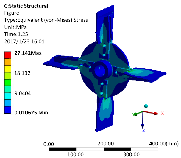
Figure 6. The equivalent stress cloud of the impeller under the loading condition

4. Fatigue Prediction for the Throwing Impeller

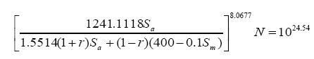
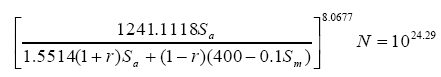
The material of the throwing impeller is Q235. It can be seen from the fatigue test data of Q235[16] that its fatigue life obeys the log normal distribution and the strength limit S_b equals 400MPa. According to Equation(1)as well as Equations(16) to (20), the S-N curve parameters can be obtained by fitting the data of the Q235 fatigue test with the least square method[19]. When the reliability is 50%, m = 8.0677 and C = 10^24.54. When the reliability is 90%, m = 8.0677 and C = 10^24.29. When the reliability is 99%, m = 8.0677 and C = 10^24.23.

Considering some factors that affect the fatigue strength of the impeller, takes K_S = 1.2, ε_S = 0.91, β = 0.85, andφ_S = 0.1[15]. Then, the Goodman-type two-parameter nominal stress fatigue life of the impeller can be solved as follows according to Equation(12).

When the reliability is 50%,

When the reliability is 90%,

When the reliability is 99%,

According to Equation (13), the Gerber-type two-parameter nominal stress fatigue life of the impeller can be solved as follows.

When the reliability is 50%,

When the reliability is 90%,

When the reliability is 99%,

According to Figure 7, the stress amplitude S_a, the mean stress S_m, and the stress ratio r at the impeller’s dangerous section can be obtained. When the throwing impeller’s reliability P is 50%, 90%, and 99%, its fatigue life at 1500r/min can be calculated respectively in Table 1 according to Formulas (12), (13),and (15). In order to evaluate the estimation accuracy of the two-parameter nominal stress model, its fatigue life prediction results are compared with those of the conventional S-N curve as well as the rating lives of the impeller in Table 1. When the conventional S-N curve is used to estimate the fatigue lives of the impeller, the random cycle load applied on the impeller has to be equivalently converted into a symmetrical cycle load.

Figure 7.

New window| Download| PPT slide

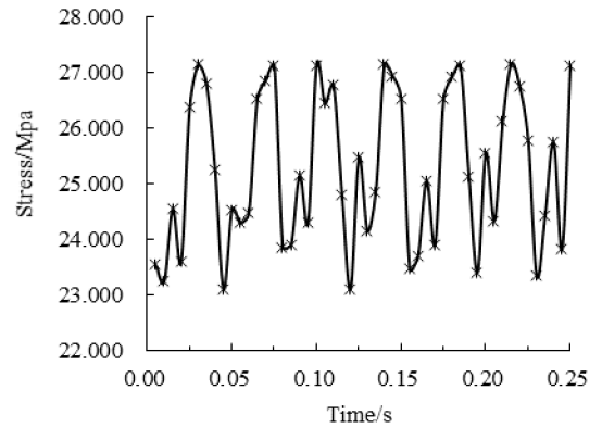
Figure 7. The stress-time variation curve at the maximum stress point of the loading impeller

Table 1. Comparisons between predictinglives and rating livesof the throwing impeller(h)

P(%)	50	90	99
Conventional S-N curve (Gerber)	1.2780×10⁷	7.1867×10⁶	6.2593×10⁶
Conventional S-N curve (Goodman)	7.7963×10⁶	4.3842×10⁶	3.8195×10⁶
Two-parameter model (Goodman)	6.1391×10⁶	3.4522×10⁶	3.0068×10⁶
Two-parameter model (Gerber)	3.2761×10⁶	1.8679×10⁶	1.6046×10⁶
Rating life	3.5×10⁶	2.0×10⁶	1.8×10⁶

New window| CSV

The comparison between the rating lives and the predicted fatigue lives of the two-parameter nominal stress model and the conventional S-N curve showed that the impeller’s actual design lives approach the calculation resultsof the Goodman and Gerber two-parameter nominal stress model. They especially come closeto those of the Gerber-type two-parameter nominal stress model and are far below those ofthe conventional S-N curve. Thismeans the estimating accuracies of the Goodman and Gerber two-parameter nominal stress models are obviously higher than those of the conventional S-N curve.

5. Conclusions

Firstly, the relational expression including the fatigue life, average stress, and stress amplitude is established by using the two-parameter nominal stress model, Miner’s fatigue cumulative damage model, and log normal distribution model of fatigue life. Its parameters can be obtained byfinite element analysis. Meanwhile, the random cycle load applied on the impeller does not have to be equivalent to a symmetrical cycle load when using the two-parameter nominal stress model to estimate the fatigue life. Theprecision of the combined method estimating the fatigue life is improved.

Secondly, the maximum stress value of the finite element calculation is slightly larger than the measured maximum stress of the throwing impeller. The relative error is 1.34%. The average stress error is 0.77%. The simulated and measured stress variation waveforms and periods are basically same. This shows that the throwing impeller’s stress simulation results are credible.

Finally, the comparisons between the rating lives and the predicted lives of the two-parameter nominal stress model and the conventional S-N curve show that the impeller’s actual rating lives are closerto the calculated livesof the Goodman and Gerber two-parameter nominal stress models than those of the conventional S-N curve. In particular, they are closer to the calculation results of the Gerber-type two-parameter nominal stress model than those of the Goodman-type two-parameter nominal stress model. This shows that the Gerber-type two-parameter nominal stress model is more accurate and suitable to predict the fatigue life of the throwing impeller.

Acknowledgements

This research is supported bythe Inner Mongolia Natural Science Foundation (No. 2018MS05059),the Inner Mongolia Talent Foundation, and the Outstanding Youth Foundation of the Inner Mongolia Agricultural University (No. 2014XYQ-9).

Reference

By original order

By published year

By cited times in this paper

By Journal Impact factor

[1]

Z. P.

Zhai

, L.

Zhou

, Z. Y.

Yang

, Y. Q.

Zhao

, S. M.

Gan

“Analysis on Vibration Characteristics of Throwing Impeller of Stalk Impeller Blower, ”

Transactions of the Chinese Society of Agricultural Engineering (Transactions of the CSAE), Vol. 31, No. 4, pp. 17-25, 2015 ( in Chinese with English abstract)

[Cited within: 1]

[2]

Z. P.

Zhai

, Y. Q.

Zhao

, H. M.

Cui

“Modal Analysis and Structure Optimization for the Throwing Impeller of the Stalk Rubbing Machine, ”

International Agricultural Engineering Journal, Vol. 25,No. 4, pp. 72-83, 2016

[Cited within: 1]

[3]

S . Chattopadhyay

and P. S. Pandey,

“Effect of Knife and Operational Parameters on Energy Requirement in Flail Forage Harvesting, ”

Agricultural Engineering Research, Vol. 73, No. 2, pp. 3-12, 1999

DOI:10.1006/jaer.1998.0395 URL [Cited within: 1]

An investigation was undertaken in the laboratory to determine the impact cutting energy while cutting single stems of forage sorghum by the knife of a flail harvesting machine. The minimum cutting speed required for complete cutting is fairly insensitive to the knife rake angle. The minimum cutting speed increased from 12·9 to 18·0 m/s for a knife rake angle range of 20 60° as the knife bevel angle was increased from 30 to 70°. Such low cutting speeds would not be capable of conveying the chopped forage successfully into the accompanying forage wagon. When the cutting speed was increased from 20 60 m/s, the cutting energy per unit cross-sectional area (specific cutting energy) for direct impact decreased by a factor of about three for bevel angles from 30 to 70°. When cutting was performed against a shear bar, the specific cutting energy drastically reduced to between one-fifth and one-fifteenth of that required for direct impact. Forward speed of the machine did not have any significant effect on specific cutting energy. The specific cutting energy is not greatly sensitive to knife rake angle, but the minimum energy requirement was observed at 40° rake angle for the experimental ranges of cutting speed and bevel angle.

[4]

S. Krzysztof and L. Aleksander,

“Two-Stage Motion of Particles in the Discharge Spout of Forage Harvester, ”

Agricultural Engineering,Vol. 124, No. 6, pp. 245-252, 2010

[5]

Lisowski

, K.Świątek, J.

Klonowski

, M.Sypuła, J.Chlebowski,

“Movement of Chopped Material in the Discharge Spout of Forage Harvester with a Flywheel Chopping Unit: Measurements using Maize and Numerical Simulation, ”

Biosystems Engineering, Vol. 111, No. 4, pp. 381-391, 2012

[6]

Z. P.

Zhai

, Z. Y.

Yang

, B.

Gao

, J. X.

“Simulation of Solid-Gas Two-Phase Flow in an Impeller Blower based on Mixture Model, ”

Transactions of the Chinese Society of Agricultural Engineering (Transactions of the CSAE), Vol. 29, No. 22, pp. 50-58, 2013 ( in Chinese with English abstract)

DOI:10.3969/j.issn.1002-6819.2013.22.006 URL [Cited within: 1]

When an impeller blower is in operation, the materials in it are conveyed mainly by means of the paddle throwing and the airflow generated by a high-speed rotating impeller blowing. In order to reveal the influence of airflow in impeller blowers on material conveying, numerical models of the air flow in the impeller blowers using the computational fluid dynamics software Fluent were developed by some scholars at home and abroad. Basic characteristics of the airflow field were obtained, which would be useful for predicting the motion of the materials. However, the studies above mentioned aimed at airflow field only, without considering materials in it, so their conclusions were not accurate. To further study the solid-gas two-phase flow mechanism in an impeller blower, a three-dimensional simulation was performed for the solid-gas two-phase turbulent flow in the impeller blower by using FLUENT software with a mixture model and a standard k- turbulence model. In the numerical calculation, the finite volume method was used to discretize the governing equations. The SIMPLEC algorithm was applied for the solution of the discretized governing equations. For the calculated zones composed of rotating impeller and static housing, Moving Reference Frames(MRF) was used to simulate the two-phase flows in complex geometries. Comparisons between the simulated values and the measured values of materials velocity at the discharge vertical pipe by high-speed video in reference paper [4] were made, and the reliability of the numerical simulation was verified. Meanwhile, on the basis of the analysis of the law of materials flow, contrast simulations on variations in working parameters such as paddle numbers, impeller's rotational speed, material-fed speed, and volume fraction of solid phase were carried out. It was concluded that: 1) The mixture model was successfully applied to simulate the turbulent particle-gas two-phase flows in an impeller blower, and predict the conveying property of the impeller blower. 2) Impellers with 4 paddles were more favorable for throwing/blowing materials than 3 and 5 paddles, because the materials velocity distribution of the middle plane(Z=0) of the impeller and the discharge pipe with 4-paddle was more even than that of 3-paddle and 5-paddle ones, and fewer vortex flows were generated. Besides, the axial symmetry of 4- paddle impeller blower was better than that of 3-paddle and 5-paddle ones, with a fine balance at a high speed, especially. 3) Distributions of materials velocity in the impeller blower did not change much with the impeller's rotational speed increasing, but the velocity of throwing/blowing materials changed much with it, and the higher the rotational speed was, the higher the velocity of throwing/blowing materials was. 4) An impeller's rotational speed and volume fraction of solid phase at the inlet being equal, feeding velocity determines the quantity of material fed into the impeller blower, and affects the distribution of volume fraction of solid phase at the impeller zone; In the limiting feed quantity range, higher feeding velocity means a larger volume fraction of solid phase and a higher velocity of throwing/blowing materials at the outlet, and was more favorable for conveying materials. 5) The change of the volume fraction of solid phase at inlet has less influence on the distribution of materials velocity; it only affects the volume fraction of solid phase at the entire zone, and the volume fraction of solid phase at the entire zone increases with the increase of material volume fraction at the inlet.

[7]

Dileep

, S. E.

Muthu

, P.

Udayanan

, R. K.

Mishra

“Multiaxial Fatigue Damage Prediction and Life Estimation of a Centrifugal Impeller for a Turboshaft Engine, ”

Journal of Failure Analysis & Prevention, Vol. 16, No. 6, pp. 883-891, 2015

DOI:10.1007/s11668-015-0032-7 URL [Cited within: 1]

ABSTRACT The complex stress/strain response of a centrifugal impeller in a Turbo-shaft engine under the multiaxial loading is analyzed using a complete thermo-mechanical finite element approach The results are processed using several multiaxial fatigue damage models like maximum von Mises strain model, maximum shear strain model, Smith Watson Topper model, Fatemi and Socie model and so on to obtain the fatigue life. In the current investigation the stress- strain unloading and the reloading behaviour consistent with a spring and slider rheological model was assumed for the fatigue life estimation. Structural integrity tests were carried out on the centrifugal impeller in order to validate the simulation results. It was found that the maximum von Mises equivalent strain approach, maximum shear strain approach and the Smith Watson and Topper criteria tend to give non conservative results. The shear strain based critical plane models suggested by Kandil, Brown and Miller and Fatemi-Socie models have showed better prediction capability and fitted the scatter band of test results within a factor of two.

[8]

E. M.

Shanmugam

, R. V.

Prakash

, S. Ammaiappan,

“Probabilistic Fatigue Life Assessment of a Titanium Alloy Impeller for Turbo Shaft Engine Application, ”

in Proceedings ofASME 2015 Gas Turbine India Conference, 2015

[Cited within: 1]

[9]

, H. J.

Cao

, H. L.

Liu

, Y. B.

Zhang

“Assessment of Fatigue Life of Remanufactured Impeller based on FEA, ”

Frontiers of Mechanical Engineering, No. 3, pp. 219-226, 2016

DOI:10.1007/s11465-016-0394-x URL [Cited within: 1]

预言重新生产的离心的压缩机 impellers 的疲劳生活是一个批评问题。在这篇论文， S-N 曲线数据被联合试验和理论推理获得。负担光谱被在修理区域基于离心的力量，剩余压力，和空气动力学的负担的全面考虑数方法的雨流动编。一个疲劳生活模拟模型被造，并且疲劳生活基于疲劳被分析累积损坏统治。尽管不能提供高精确的预言，模拟结果为疲劳生活影响因素和疲劳破裂区域的分析是有用的。结果证明负担振幅极大地影响了疲劳生活， impeller 被保护免受在超速跑的伤害，并且预言的疲劳生活以评估速度安全地在下一个服务周期以内满足。

[10]

Liao

, H. Z.

Huang

, S. P.

Zhu

, D.

Ling

“Turbine Disk Fatigue Life Prediction based on Generalized σ-N Surface, ”

Journal of University of Electronic Science and Technology of China, Vol. 42, No. 2, pp. 316-320, 2013

[Cited within: 1]

[11]

D. G.

Pavlou

“The Theory of the S-N Fatigue Damage Envelope: Generalization of Linear, Double-Linear, and Non-Linear Fatigue Damage Models, ”

International Journal of Fatigue,Vol. 110, pp. 204-214, 2018

DOI:10.1016/j.ijfatigue.2018.01.023 URL [Cited within: 1]

A new theory for macroscopic fatigue damage estimation based on the S-N curve is presented. The proposed concept assumes that the area bounded by the S and N axes, and the S-N curve, can provide a characteristic damage map for each material. Finite element analysis is used to derive colored damage zones and non-linear isodamage lines within the S-N fatigue damage envelope. Implementation of this theory on two arbitrarily selected alloys under stepwise variable stresses is provided, and the successful prediction of the remaining life is discussed. The proposed S-N fatigue damage envelope theory is a generalization of most of the existing fatigue damage models.

[12]

Saggar

, H.Sallem, C.

Bouraoui

“Fatigue Life Prediction under Variable Loading based on a New Damage Model Devoted for Defective Material, ”

International Journal of Advanced Manufacturing Technology, Vol. 95, No.1- 4, pp. 431-443, 2018

DOI:10.1007/s00170-017-1198-9 URL [Cited within: 2]

This article presents a fatigue damage cumulative model under variable loading devoted for defective materials. The multiaxial stress amplitude is reported to the equivalent stress by combining it wit

[13]

M. L.

Aggarwal

, V. P.

Agrawal

, R. A.

Khan

“A Stress Approach Model for Predictions of Fatigue Life by Shot Peening of EN45A Spring Steel, ”

International Journal of Fatigue, Vol. 28, No. 12, pp. 1845-1853, 2006

DOI:10.1016/j.ijfatigue.2005.12.004 URL [Cited within: 1]

A lot of research has been done to improve fatigue strength of materials by creating compressive residual stress field in their surface layers through shot peening. In this paper, fatigue strength of shot peened leaf springs has been calculated from laboratory samples. The axial fatigue strength of EN45A spring steel specimen is evaluated experimentally as a function of shot peening in the conditions used for full-scale leaf springs testing in industries. Optimum shot peening condition for specimen is found and S/ N curves of the specimens are correlated with leaf springs curve. A mathematical model has been developed which predicts the fatigue life of leaf springs for a given stress at varying shot peening conditions. Predictions from this model are compared with experimental data. The estimation of fatigue life and relaxation of compressive residual stress field are discussed.

[14]

Ishihara

, A. J.

Mcevily

, M.

Sato

, K

Taniguchi

, T

Goshima

“The Effect of Load Ratio on Fatigue Life and Crack Propagation Behavior of an Extruded Magnesium Alloy, ”

International Journal of Fatigue, Vol. 31, No.11- 12, pp. 1788-1794, 2009

DOI:10.1016/j.ijfatigue.2009.02.034 URL [Cited within: 1]

Fatigue experiments were carried out in laboratory air using an extruded magnesium alloy, AZ31, to investigate the effect of load ratio on the fatigue life and crack propagation behavior. The crack propagation behavior was analyzed using a modified linear elastic fracture mechanics parameter, M. The relation crack propagation rate vs. M parameter was found to be useful in predicting fatigue lives at different R ratios. Good agreement between the estimated and the experimental results at each stress ratio was obtained.

[15]

S. Z.

Zhou

, K. Q.

Zhu

, H.

C . Wu

, and C. Qiao,

“Fatigue Life Analysis of the BlenderTruck Mixing Impeller based on Workbench, ”

China Petroleum Machinery,No. 2, pp. 36-38, 2012

[Cited within: 2]

[16]

J. L.

Fan

, X. L.

Guo

, C. W.

, and D. W.

Deng

“Fast Evaluation of Fatigue Behavior of Q235 Steel by Infrared Thermography and Energy Approach, ”

Journal of Materials Engineering,Vol. 40,No. 12, pp. 71-76, 2012

[Cited within: 2]

[17]

W. X.

Liu

, “Mechanical Reliability Design, ”Tsinghua University Press, Beijing, 1996

[Cited within: 1]

[18]

Z. P.

Zhai

, L.

Zhang

, C. Z.

Liu

, H.

N . Li

, and H. M. Cui,

“Numerical Simulation and Experimental Validation of Radiation Noise from Vibrating Shell of Stalk Impeller Blower, ”

Transactions of the Chinese Society of Agricultural Engineering (Transactions of the CSAE), Vol. 33, No. 16, pp. 72-79, 2017 (in Chinese with English abstract)

DOI:10.11975/j.issn.1002-6819.2017.16.010 URL [Cited within: 2]

Stalk rubbing machine is a new type of forage processing equipment developed in China.It is mainly composed of rubbing device and impeller blower.When the stalk rubbing machine is working, the material is thrown out by the impeller blower after rubbed by the rubbing device.Its main problem is an increased level of vibration and noise of the impeller blower during the stalk rubbing machine running.However, the research of impeller blowers at home and abroad mainly focused on reducing the power consumption, increasing the throwing distance and throwing efficiency.There were few researches on reducing the vibration and noise of the impeller blowers.Because of the limitation of the experimental method, it was difficult to find out how the shell was excited by the pulsating gas-solid two-phase flow inside the impeller blower and how it produced vibration and radiated noise outwards.Aimed at these problems, the vibration radiated noise of the shell of the impeller blower was analyzed by the co-simulation method to predict the impeller blower's noise at the design stage of the stalk rubbing machine.Firstly, the ANSYS Fluent software was used to simulate the unsteady solid-gas two-phase turbulent flow in the impeller blower.Then the fluctuating pressure of the two-phase flow field was loaded into the inner surface of the shell.Secondly, the modal analysis and dynamic response analysis of the shell were carried out by using the finite element method which realized unidirectional coupling from gas-solid two-phase fluid to structure.With the vibration response of the shell as the acoustic boundary condition, the vibration radiation noise of the shell caused by unsteady flow was calculated by using the indirect boundary element method(IBEM) of the LMS Virtual Lab.Thirdly, Comparisons between the simulated values and the measured values of the vibration radiation noise of the shell were made, and the reliability of the numerical simulation was verified.Finally, the influence of shell thickness on the vibration radiation noise was analyzed based on the above co-simulation method.Research results showed that:1) The fundamental frequency sound pressure levels for the simulation and experiment were basically the same.The changing trends of simulation results and the experimental results of the fundamental frequency and harmonics were also the same.Because the simplified simulation model made its stiffness smaller, the simulation results at the second and the third harmonic were slightly higher than the experimental results.Thus, it could be proved that the results of the co-simulation were credible.2) The fundamental frequency sound pressure level was the highest.The second harmonic one came second, the third harmonic one was low, and the rest harmonic ones were very low and were neglected.3) The sound pressure level of the radiated noise at the sides of the shell was the highest, particularly at inlet.And it was higher at outlet, too.4) When the impeller rotational speed was 1 500 r/min, the best wall thickness was the combination of front and rear round shell thickness of 4 mm and the others' thickness of 3 mm.The research will provide the reference for further research on the noise of stalk rubbing machines and impeller blowers.

[19]

J. L.

Fan

, X. L.

Guo

, C.

W . Wu

, and Y. G.Zhao,

“Research on Fatigue BehaviorEvaluation and Fatigue Fracture Mechanisms of Cruciform Welded Joints, ”

Materials Science & Engineering A,Vol. 528, No. 29- 30, pp. 8417-8427, 2011

[Cited within: 1]

“Analysis on Vibration Characteristics of Throwing Impeller of Stalk Impeller Blower, ”

2015

... An impeller blower generally consists of the throwing impeller, shell, and discharge tube. This device is widely used to convey materials in various forage harvesters because of its simplicity, reliability, easy maintenance, high capacity, and low manufacturing cost [1]. As the core working component, the throwing impeller often endures the combined action of the centrifugal force, the gravity, and the varying pressure of high-speed air flow and materials inside the impeller blower. This will accelerate the throwing impeller’s fatigue, leading to fracture [2]. In recent years, most research on impeller blowers mainly focused on reducing the power consumption as well as increasing the throwing distanceand efficiency [3-6]. However, relatively few data exist on the topic of investigating the fatigue life of the throwing impeller. Thus, it is very necessary to find a feasible model to accurately estimate the fatigue life of throwing impellers. ...

“Modal Analysis and Structure Optimization for the Throwing Impeller of the Stalk Rubbing Machine, ”

2016

“Effect of Knife and Operational Parameters on Energy Requirement in Flail Forage Harvesting, ”

1999

“Two-Stage Motion of Particles in the Discharge Spout of Forage Harvester, ”

2010

“Movement of Chopped Material in the Discharge Spout of Forage Harvester with a Flywheel Chopping Unit: Measurements using Maize and Numerical Simulation, ”

2012

“Simulation of Solid-Gas Two-Phase Flow in an Impeller Blower based on Mixture Model, ”

2013

“Multiaxial Fatigue Damage Prediction and Life Estimation of a Centrifugal Impeller for a Turboshaft Engine, ”

2015

... Research works on the fatigue life for the similar rotating machine are presented as follows.Dileep [7] estimated the low-cycle fatigue life of a centrifugal impeller under the engine operating conditions by using four different multi-axial fatigue damage models. The predicted lives were then compared with the experimental value obtained from the cyclic spin test. The critical plane-based models showed better prediction accuracy and capability in comparison to the maximum von Mises strain range model. Shanmugam[8] estimated the fatigue life of a titanium alloy centrifugal impeller by using the equivalent strain method and Smith Watson Topper (SWT) method and assessed the fatigue life via the cyclic spin test. The probabilistic analysis of fatigue life was carried out by using the Weibull distribution method. It was found that the equivalent strain method is nonconservative due to the exclusion of the mean stress effect. The average fatigue life of the impeller was estimated at 12000 cycles by using the SWT method, which was closer to the test results. Xu[9] analyzed the fatigue life of a remanufactured centrifugal compressor impellers by using the S-N curve data and the rain-flow counting method based on FEA. It was found that the simulation results were useful for analyzing fatigue life impact factors and fatigue fracture areas, although it was incapable of providing high-precision prediction. Liao and Huang[10] investigated the fatigue life of a turbine disk by constructing Goodman and Gerber types of a generalized σ-N curved surface equation based on stress amplitude and mean stress. An aircraft engine turbine disk was presented to validate the proposed method. The results showed that the prediction of the Goodman equivalent life curve was much more accurate than that of the Gerber type model. This method also showed better accuracy for estimating the fatigue life than the conventional S-N curve. Pavlou [11] presented a new theory for macroscopic fatigue damage estimation based on the S-N curve, which was a generalization of most of the existing fatigue damage models. Saggar [12] presented a fatigue damage cumulative model under the variable load devoted for defective materials. This model was connected cycle by cycle with the S-N curve, and it also took into account the loading history. The predicted results of this model were compared with the experimental results for a C35 low alloy steel containing defects and those computed by Miner’s model. It was demonstrated that the proposed model predicted the fatigue damage much better than the Miner rule. ...

“Probabilistic Fatigue Life Assessment of a Titanium Alloy Impeller for Turbo Shaft Engine Application, ”

2015

“Assessment of Fatigue Life of Remanufactured Impeller based on FEA, ”

2016

“Turbine Disk Fatigue Life Prediction based on Generalized σ-N Surface, ”

2013

“The Theory of the S-N Fatigue Damage Envelope: Generalization of Linear, Double-Linear, and Non-Linear Fatigue Damage Models, ”

2018

“Fatigue Life Prediction under Variable Loading based on a New Damage Model Devoted for Defective Material, ”

2018

... According to the S-N curve and the constant life curve of material, the two-parameter nominal stress equation including the average stress S_m, the stress amplitude S_a, and the fatigue life N can be deduced as follows [12-13]. ...

“A Stress Approach Model for Predictions of Fatigue Life by Shot Peening of EN45A Spring Steel, ”

2006

“The Effect of Load Ratio on Fatigue Life and Crack Propagation Behavior of an Extruded Magnesium Alloy, ”

2009

... If we choose the Gerber formula as the constant lifecurve [14], ...

“Fatigue Life Analysis of the BlenderTruck Mixing Impeller based on Workbench, ”

2012

... If we apply the S_a-S_m-N two-parameter nominal stress models of material into estimating the fatigue life of the actual throwing impellers, the factors including the stress concentration, size, surface quality, and sensitivity of impeller material to the asymmetrical cycle stress that affect the fatigue strength of the impeller must be considered[15]. The revised Goodman-type two-parameter nominal stress equation is listed as follows: ...

... Considering some factors that affect the fatigue strength of the impeller, takes K_S = 1.2, ε_S = 0.91, β = 0.85, andφ_S = 0.1[15]. Then, the Goodman-type two-parameter nominal stress fatigue life of the impeller can be solved as follows according to Equation(12). ...

“Fast Evaluation of Fatigue Behavior of Q235 Steel by Infrared Thermography and Energy Approach, ”

2012

... Due to the randomness of the basic variables such as load, material parameters, and geometrical parameters of the impeller in the working process, the fatigue life shows discreteness. The throwing impeller’s material is Q235, and its fatigue life distribution obeys the log normal distribution according to the existing research [16]. ...

... The material of the throwing impeller is Q235. It can be seen from the fatigue test data of Q235[16] that its fatigue life obeys the log normal distribution and the strength limit S_b equals 400MPa. According to Equation(1)as well as Equations(16) to (20), the S-N curve parameters can be obtained by fitting the data of the Q235 fatigue test with the least square method[19]. When the reliability is 50%, m = 8.0677 and C = 10^24.54. When the reliability is 90%, m = 8.0677 and C = 10^24.29. When the reliability is 99%, m = 8.0677 and C = 10^24.23. ...

1996

... Under the action of the cyclic load, the distribution law of the impeller’s fatigue life can be expressed by the log normal probability density function [17]as follows: ...

“Numerical Simulation and Experimental Validation of Radiation Noise from Vibrating Shell of Stalk Impeller Blower, ”

2017

... The three-dimensional modelling software Pro/E is used to build a three-dimensional solid model of the impeller. The three-dimensional solid model of the impeller is then imported into HyperMesh for meshing. The numbers of cells and nodes of the entire impeller model inthe finite element mesh are 26, 800 and 40, 532 respectively [18]. ...

... Based on the numerical calculation results under the unloaded condition, the numerical calculation of the gas-solid two-phase unsteady flow in the impeller blower under the loading condition is carried out by using the large-eddy simulation and the dense-discrete phase model. The pressure distribution of material and air flow to the impeller is obtained[18]. Similarly, the Fluent and Workbench coupling platform in the Workbenchis used to exert the airflow-material two-phase flow field pressure on the coupling surface of the impeller in the numerical calculation. The rest of the numerical calculations are the same as the unloaded condition mentioned above. ...

“Research on Fatigue BehaviorEvaluation and Fatigue Fracture Mechanisms of Cruciform Welded Joints, ”

2011

〈

〉