Many researchers have studied viscoelastic material parameter fitting. Bradshaw and Brinsonfitted related parameters in the linear viscoelastic solid using a signal control method [1]. Yin analysed the curve fitting method to determine the viscoelastic material stress-strain relationship of the five constants and drew a corresponding fitting formula [2]. Li analysed experimental data to show that the fractional derivative model can substitute for a number of Prony series so that the calculation is relatively simple[3]. Jimenez et al. studied the stress relaxation parameters of two different kinds of polymer fitting under the conditions of constant temperature and strain by the generalized Maxwell model [4]. Huang and Yin analysed the fitting results of some viscoelastic damping materials and simplified the original fitting formula. This reduced the difficulty of using the curve fitting method to determine constants [5]. Duan et al. fitted the generalized Maxwell model of viscoelastic material by the Kohlrausch-William-Watts (KWW) function method of the minimum[6]. Zhan et al.analysed the performance of the linear viscoelastic generalized Maxwell model and dynamic viscoelasticity of the fractional order derivative Maxwell model, showing thatthe fractional order derivative of the fitting effect was better than others [7]. Wei et al. studied the cartilage of viscoelastic material using the method of numerical fitting and deduced the relationship between the normalized experimental curve of the simplified model and the generalized Maxwell model.The rib cartilage materials were used for viscoelastic finite element analysis of Maxwell model parameters [8]. At the same time, Yin et al.determined that fractional order calculus can be used to describe the asphalt mixture of fractional derivative viscoelastic constitutive relation, and they obtained good fitting effects[9]. Shekhar and Sahasrabudhe proposed the fluid Maxwell viscoelastic model for solid rocket propellant, which can predict some material coefficients of solid rocket propellant through a uniaxial tensile experiment [10]. Haario et al. recognized viscoelastic parameters of the polymer model usingthe Markov chain Monte Carlo (MCMC) method [11].

Neural networks in the parameter fitting of viscoelastic materials also have many applications.Gasperlin et al. put forward predicting the viscoelastic behaviour of emulsion systems through a neural network based mathematical model. It had certain precision [12]. Zeng and Shu gave an equivalence relation of a three layer delay feed forward neural network to the Green Rivlin nonlinear viscoelastic constitutive equation, which solved the nuclear function by the network in various order of the G R equation. They pointed out that the neural network method can be widely applied to the material constitutive relation research [13]. Al-Haik et al. studied the stress relaxation behavior of polymer composites based on artificial neural networks. They accurately predicted a wider range of nonlinear viscoelastic models[14]. Saeidirad et al. studied the viscoelastic behavior of pomegranates with an artificial neural network, and the predicted results were more accurate [15]. Zheng et al.studied the method of whole loading process of relaxation modulus based on a genetic algorithm to accurately obtain the viscoelastic constitutive parameters of HTPB composite solid propellant [16].

Obtaining the viscoelastic material parameter fitting expression is an issue that has received much attention, and the traditional method is unable to create a neural network according to the specific problems. Aiming at this, a custom neural network is applied to fitting and issimple, effective, and accurate.

The remainder of this paper is outlined as follows. Section 2 discusses Prony series expression of viscoelastic material performance parameters. In Section 3, weconstructa custom neural network based on Pronyseries. In Sections 4 and 5, anumerical example is introduced and the resultsare analysed. Finally, Section 6 concludes with recommendations for future work.

The Maxwell model or generalized Kelvin model are commonly used in the analysis of viscoelastic stress (strain). Because the combination of the elastic element and the cohesive element is increasingly complicated, the stress-strain relationship of the model, or the constitutive relation, can better reflect the actual situation of viscoelastic material. In general, we often use the generalized Kelvin model to inspect the creep effects of viscoelastic materials, and we use the generalized Maxwell model to observe the relaxation effect of viscoelastic materials. This article is aimed at fitting the relaxation modulus; therefore, it elaborates on the generalized Maxwell model in detail.

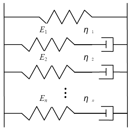
The multiple Maxwell model and a spring in parallel is the generalized Maxwell model, as shown in Figure 1, where E_i is the elastic modulus of the i^th original elastic and ${{\eta }_{i}}$ is the viscosity coefficient of the i^th original viscosity. Each Maxwell model of the stress-strain relationship is $\dot{\varepsilon }\text{=}{{\sigma }_{i}}/{{\eta }_{i}}+{{\dot{\sigma }}_{i}}/{{E}_{i}}$. By differential operator, the stress ofexpressionis${{\sigma }_{i}}=\frac{{{E}_{i}}{{\eta }_{i}}}{{{E}_{i}}+{{\eta }_{i}}D}D\varepsilon $, $D=d/dt.$ Adding up the stress of each Maxwell model, the spring stress is the total stress of the generalized Maxwell model [17-18], that is,

${{\sigma }_{e}}$ is referred to as the equilibrium parameter, as shown in Figure 1.

References [18-19] provided the derivation process forthe constitutive relation and integral constitutive relation of the generalized Maxwell model. The expression of the relaxation modulus of $Y(t)$ is

Where $Y(t)$ is the relaxation modulus of each Maxwell model and ${{Y}_{e}}$ is the equilibrium parameter.Equation (2) is expressed in the Prony series of the relaxation modulus, elaborating all the meanings in the following paragraphs.

In the traditional fitting method, we use the Prony series fitting method to fitting the material relaxation modulus, and selecting a low number leads to poor fitting precision. However, if an infinite number is takenin order to pursue precision, this instead complicates the expression and makes fitting difficult. The fractional derivative model fitting has higher fitting precision than the Prony series, and the fitting parameters are less than those of the Prony series. However, the fractional derivative model also has some disadvantages, such as a complex constitutive equation derivation process, and the Mittag-Leffler function in the selection of the series number determines the complexity of the constitutive equation [18]. The neural network has the ability to gain any function approximation with any degree of accuracy; thus, it has been widely used in function fitting.

The traditional neural network usually useslogsig general functions and the tansig function as the transfer function of neurons. It can act as a general function approximation. Its disadvantage is that the traditional neural network model does not correspond to the physical model (fitting formula), so the generalization ability is poor. Though the traditional transfer function involves repeated verification by people, it has better accuracy, stability, and strong calculation, and it can be applied tomost data calculations. However, its calculation process and fitting formula are renegade and cannot correspond with a specific calculation formula.

To address this, the instance analysis below uses a custom neural network. The transfer function is based on a specific formula of Equation (2) and combines the neural network and fitting formula together. The neural network weights and threshold can correspond to the elasticity modulus and viscosity coefficient. We can obtain parameters of the generalized Maxwell model from training after the network structure, providing convenience for engineering practice.

A neural network is created by a standard toolkit network that creates functions and corresponds to a certain network type. However, different learning training algorithms will not be able to use the standard function to create. This requires the application of a custom network method. A custom network is implemented by invoking the network function. The network object contains many properties, thereby changing the network structure, algorithm, function, etc. Reference [20] gives a specific custom neural network program.

Our purpose isto use the neural network structure created material relaxation modulus expression. The Prony series serves as an effective form of relaxation modulus. Therefore, we should consult the Prony series to determine the form of the structure of the network. Referencing Equation (2), the shear modulus of Prony series can be expressed as

Where ${{\tau }_{i}}={{\eta }_{i}}/{{G}_{i}}$, ${{G}_{e}}=G(\infty )$, and $G(\infty )$ are the equilibrium modulus, ${{G}_{i}}$ is the shear modulus of elasticity of each Maxwell model, and ${{\eta }_{i}}$ is the viscous coefficient [21].

In Equation (3), firstly, t independent variables are calculated through the weighted index, followed by the index proceeded linear weighted superposition. This structure is similar to the neural network structure. With this characteristic, the network weights correspond to the weighted coefficient and the network thresholds correspond to the constant term in the formula. We regard the exponential function as the network transfer function. Because of the rationality of the Pronyseries fitting, the custom neural network fitting method for shear modulus is a reasonable method. The following custom concrete structure of the neural network is presented.

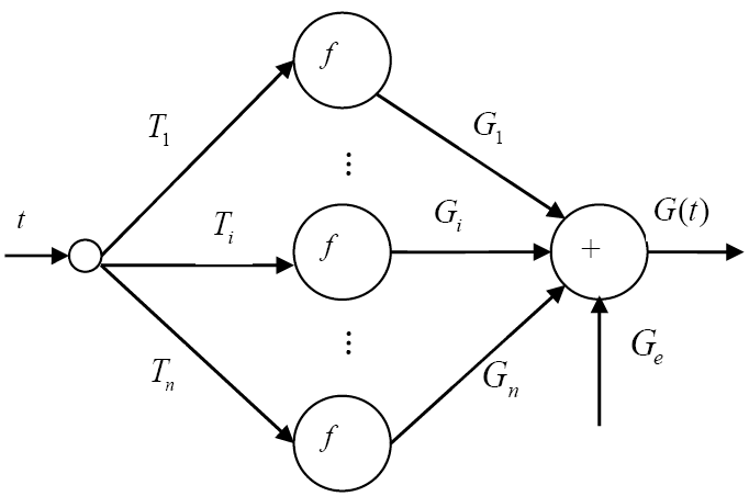
The network shown in Figure 2 has three layers. Among them, the input layer and output layer include one input unit, and the number of hidden layer neurons determines the series number of the Prony series. t(time) is the input, and $G(t)$ (shear modulus) is the output. ${{T}_{i}}=1/{{\tau }_{i}}$ is the weight between the input layer and hidden layer, and the threshold of the hidden layer is set to none by the unique function of custom neural networks. ${{G}_{i}}$ is the weight between the hidden layer and output layer, and ${{G}_{e}}$ is the threshold of the output layer. The transfer function of hidden layer neurons is an exponential function whose expression is $f={{e}^{-x}}$. The transfer function of neurons in the output layer is purelin, that is, a linear transfer function.

According to the above three layers of custom neural network structure, in the network learning process, the calculation formula for the neural network hidden layer unit output value is

The calculating formula for the output layer is

In this paper, we use the mean square error function as the performance function of the neural network. It is used to evaluate the difference between the actual network output and the target, and the formula is given in [13]. For q samples of network output, the form is

where $A(j)$ is the j^th expected value of the network output sample.

The L-M training algorithm is used to adjust network weights and thresholds. When the network converges, the network weights and thresholds can be transformed into coefficients in the Prony series of viscoelastic material shear modulus to complete the material model modelling.

As a standard example, a viscoelastic material shear modulus changes over time in the case of constant temperature, as shown in Table 1. A part of experimental data isused to train the neural network. Another part of experimental data is used to test the calculation results of the neural network.

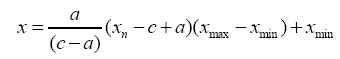
Based on the above data structure of neural network training samples, because the order of magnitude of data gap islarger, we normalize processing to facilitate the training of the neural network and data processing. The neural network’s input and output data are normalized in the range of [a, c]. The normalization formula is

where $x$ is the original data, ${{x}_{n}}$ is the data of normalization, ${{x}_{\min }}$the is minimum value of the original data, and ${{x}_{\max }}$ is the maximum value of the original data.

After completion of the neural network training and simulation, the normalized data reverse the original data. The reverse normalization formula is

(8)

According to the above example, because the parameters are positive values in the Prony series, the neural network’s weights and thresholds correspond to the parameters in the Prony series. Therefore, in order to ensure that the neural network weights and thresholds are positive values, take a = 1 and c = 11.

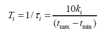
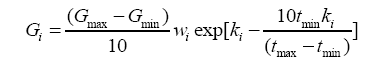
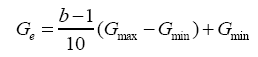
After training of the custom neural network, use mathematical derivation of the weights and thresholds after training to obtain the weights and threshold before normalization. This is each parameter of the Prony series. The formula is

(9)

(10)

(11)

Where k_i is the weight between the input layer and hidden layer (vector), w_i is the weight between the hidden layer and output layer (vector), andbis the threshold of the output layer.

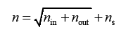
When the neuron number of hidden layer is n,the empirical Equation[21] is

(12)

Where n_in s the neuron number of the input layer, ${{n}_{\text{out}}}$ is the neuron number of the output layer, and ${{n}_{\text{s}}}$ is constant for [1,10].

For the above example, the neuron number of the hidden layer was taken as $n=2, 3,\cdots , 11.$ Through repeated training, the simulation results of different neuron numbers of the hidden layer are compared. We obtained the proper neuron number of the hidden layer.

The experimental data is divided into training set and test set. We useten groups as the training set and six groups as the test set. The training set is shown in Table 2. At the same time, new data can also be added to train and test.

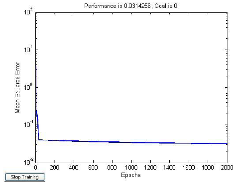
Take $n=2, 3,\cdots , 11$ and the transfer function of hidden layer neurons as $f={{e}^{-x}}.$ After training 2000 steps, the maximum relative error of the test set and each parameter value of the corresponding Prony series can be calculated, and they are listed in Table 3.

As can be seen from Table 3, the error is minimized when the neuron number is 3. When the number of neurons increases, the error continues to increase. According to the above results, the maximum relative error of the test results is small, which shows that the network weights and threshold achieved good fitting results.

Using the training samples in Table 2, the number of hidden layer units is taken as $n=2, 3,\cdots , 11$. The maximum relative error calculated by the BP neural network method after training 2000 steps is shown in Table 4.

Prony series fitting is done by using the same training samples through the Prony series fitting method in Ansys software. When the number of items is taken separately as $n=1, 2,\cdots , 4$, the maximum relative error in the test sample is shown in Table 5.

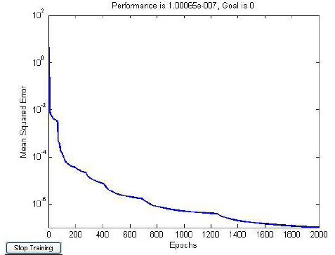
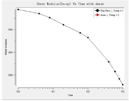
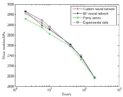
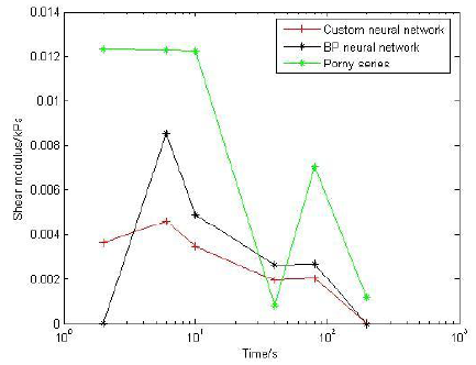
In order to facilitate comparison, the above three fitting methods are taken simultaneously as $n=3$, and the training error convergence curves of the custom neural network and BP neural network are respectively shown in Figures 3 and 4. The fitting curve of the Prony series in the Ansysis shown in Figure 5. Through the simulation of test sample points, the calculation results of the shear modulus are shown in Table 6. Figure 6 shows the comparison between the calculated results of test sample points and the experimental data. The maximum relative error is shown in Figure 7.

It can be seen from the simulation results in Table 6 that the error of the traditional BP neural network method is larger than that of the proposed method in this paper. Therefore, the results of the custom neural network method are acceptable. However, the weights and thresholds of the BP neural network cannot correspond to the elastic modulus and viscous coefficient of the generalized Maxwell model, and the concrete structure of the generalized Maxwell model cannot be inversely derived. This is a major drawback of traditional neural network parameter fitting. However, the exact parameters of the generalized Maxwell model can be inversely deduced while the method of custom neural network is used to accurately fit the shear modulus.

As shown in Table 6, when the Prony series term is 3, the maximum relative error is 1.24%. Through the results, it can be seen that the maximum relative error in each fitting point of this method is larger than the maximum relative error of the neural network calculation under the same fitting terms. As shown in Table 5, the higher the number of chosen Prony series, the more complicated the calculation process.

Through the generalized Maxwell model of viscoelastic material Prony series fitting research, we found a custom neural network method to fit the relaxation modulus of viscoelastic materials. The custom neural network can select the transfer function, weights, and threshold according to the particular form of expression, and the neural network also has specific physical meaning. Through the example analysis, the custom neural network training error is shown to be smaller, and the convergence is faster. The test results also showed that the weights and thresholds of the neural network model, namely the fitting of the shear modulus and viscosity coefficient, reached a very high accuracy. The parameters in the generalized Maxwell model can be obtained from the trained network to facilitate the engineering practice.By the same theory, the creep compliance of the generalized Kelvin model can also be fitted in the same way. Therefore, it is a good method to fit the modulus compliance and other parameters of viscoelastic materials using a limited set of samples after training the neural network.

This researchis supported by the National Natural Science Foundation of China (No. 11262014).