


1. Introduction
Portfolio selection problem is concerned with the optimal allocation of one’s wealth to obtain maximum profitable return and bear minimum risk control. Since Markowitz [1] published the classic MVM that has served universally as a pioneering portfolio selection model over the past several decades, many researchers have proposed numerous variants of the MVM by adding new methods or new elements that are all based on probability theory and mathematical statistics theory. Unfortunately, the securities market is often complex, and there is not enough historical data to reflect the volatility of the future securities market in some real-world cases. To address this case, more and more portfolio selection approaches based on fuzzy theory have been proposed. The security returns are regarded as fuzzy variables that rely on experienced experts’ evaluations instead of historical data. However, paradoxes are produced when using fuzzy variables to describe the subjective estimations of security returns [2]. In order to eliminate this contradiction, Liu [3] proposed an uncertain measure and further developed the uncertainty theory, an approach that has been widely used in various areas. It has also been introduced to address the portfolio optimization problem. It is worth noting that some scholars have taken the risk-free asset into consideration in uncertain portfolio optimization [4-5]. This is an interesting and different approach from those seen in the above works in the use of risk measurement. Huang [4] first proposed a risk index model, and Huang and Qiao [5] further modeled the multi-period portfolio selection problem. These works verified that the above-mentioned paradoxes will disappear immediately when describing the human imprecise estimations of security returns as an uncertain variable [4-5].
There is a fact that existing research usually tends to ignore the function of risk-free assets for investors, and the investor’s wealth allocation is usually too decentralized or centralized. To make up for this deficiency, Gao and Liu [6] first proposed a RFPI model for uncertain portfolio selection. They no longer considered only the weight of risk assets and made sure that investors do not put their eggs into one basket via an entropy constraint. They found that investors can set up a suitable confidence level and a minimum FRPI value subjectively. However, many investors lack professionalism in investment and have an ambiguous risk preference or other subjective and objective factors such that the threshold of RFPI’s preset value cannot accurately be determined in reality. In this paper, based on RFPIEM, we develop a new RFPI model for uncertain multi-objective portfolio selections with entropy and variance constraints. Firstly, we develop a new risk-free protection index model for multi-objective portfolio selections. We not only take the expected return maximization as the first objective function but also maximize RFPI as the second objective function to fully make its protective effect of risk-free assets on risk assets work. Secondly, we further take proportion entropy and variance constraints into consideration to measure portfolio diversification. Finally, we give an example analysis and also show a comparison between the multi-objective uncertain portfolio model with entropy constraint and the model without entropy constraint and a comparison between the multi-objective uncertain portfolio model with FRPI maximization and MVM. The model with FRPI maximization added as the second objective function is better than the MVM for multi-objective portfolio selection.
The rest of the paper is organized as follows. Section 2 briefly reviews some properties of uncertain variables and entropy constraint in finance. In section 3, we first present Huang’s risk index model (RIM) and Gao and Liu’s risk-free protection index-entropy model (RFPIEM) for uncertain portfolio briefly. Then, we further propose a risk-free protection index model with entropy and variance constraints for multi-objective uncertain portfolio selection and give an algorithm to solve the multi-objective uncertain portfolio selection by using the Delphi method. In section 4,an illustrative example is given, and a comparison between the multi-objective uncertain portfolio model with entropy constraint and the model without entropy constraint and a comparison between the multi-objective uncertain portfolio model with FRPI maximization added as the second objective function and MVM are also shown. Section 5 summarizes the conclusion.
2. The Uncertain Measure, Uncertainty Space, and Distribution of an Uncertain Variable
To suppose that security returns are uncertain variables, this section introduces some necessary knowledge about the uncertainty theory. The definition of an uncertain measure was presented by Liu [3]. Let $\Gamma $ be a nonempty set. Eachelement $\Lambda \in \zeta $ is an event in the $\sigma $-algebra $\zeta $ over $\Gamma ,$ and $M\{\Lambda \}$ is the occurrence possibility measure of $\Lambda $. The set function $M$ is called an uncertain measure if it satisfies the normality, self-duality, monotonicity, and countable subadditivity axioms:
i) Axiom 1(Normalityaxiom) $M\{\Gamma \}=1$ for the universal nonempty set $\Gamma $;
ii) Axiom2(Self-dualityaxiom) $M\{\Lambda \}+M\{{{\Lambda }^{c}}\}=1$ for ${{\Lambda }_{1}}\subset {{\Lambda }_{2}}$;
iii) Axiom 3(Monotonicity axiom) $M\{{{\Lambda }_{1}}\}\le M\{{{\Lambda }_{2}}\}$ for each event $\{{{\Lambda }_{i}}\}$;
iv) Axiom 4(Countable subadditivity axiom) $M\{\underset{i=1}{\overset{\infty }{\mathop{\cup }}}\,{{\Lambda }_{i}}\}\le \sum\limits_{i=1}^{\infty }{M\{{{\Lambda }_{i}}\}}$ for each event $\{{{\Lambda }_{i}}\}$.
The definition of an uncertainty space and an uncertain variable is given in literature [3]. Let $M$ be an uncertain measure. Then, the triplet $(\Gamma ,\zeta ,M)$ is called an uncertainty space. An uncertain variable is a measurable function from an uncertainty space $(\Gamma ,\zeta ,M)$ to $\xi $:$(\Gamma ,\zeta ,M)\to \Re $. The uncertain distribution is defined as $\Phi (x)=M\{\xi \le x\}$, $\Phi :\Re \to [0,1]$.
The expected value of an uncertain variable $\xi$ is defined as
Provided that at least one of two integrals exist. Its variance is defined as
The uncertainty distribution $\Phi \left( x \right):\Re \to \left[ 0,1 \right]$ of an uncertain variable $\xi$ is defined as
An uncertain variable $\xi $is called a normal uncertain variable if it satisfies
Which is denoted by $N\left( e,\sigma \right)$ with two real numbers $e,\text{ }\sigma $, and $\sigma >0$. If the expected value $E\left( \xi \right)$ of an uncertain variable $\xi$ exists, then
Where $\alpha \in (0,1)$. From Formula (4), we can obtain ${{\Phi }^{-1}}(\alpha )$(i.e.,the inverse function of$\Phi $):
3. A RFPI Model for a Multi-Objective Uncertain Portfolio
It is well known that the investors’ maximum tolerable variance level will be different based on different expected values [4]. In other words, it is difficult to obtain a maximum tolerable variance level when using variance as a risk measure for the portfolio selection problem. Meanwhile, it is easy to estimate the tolerable variance level of risk-free assets. Huang [4-5] first added risk-free assets to the portfolio selection problem and put forward RIM for an uncertain portfolio. However, the focus was on the allocation weight of risk assets and not the allocation of the investment proportion to the risk-free assets. Gao and Liu [6] found that risk-free assets and risk assets are both available for investors and developed RFPIEM for an uncertain portfolio. In this section, based on RIM and RFPIEM for an uncertain portfolio, we will follow the work of Gao and Liu [6] and further explore the protective effect of risk-free assets on the risk assets in an uncertain environment. We will propose a RFPI model with entropy and variance constraints for multi-objective uncertain portfolio selection in subsection 3.1 and give an algorithm to solve the multi-objective uncertain portfolio selection by using the Delphi method in subsection 3.2.
3.1. A RFPI Model for a Multi-Objective Uncertain Portfolio Selection with Entropy and Variance Constraints
In Gao and Liu’s work [6], it supposed that the investors must determine a preset minimum FRPI value according to their risk preference and risk tolerance. In other words, a suitable confidence level and the preset threshold value of FRPI are predetermined subjectively by investors before making their portfolio selections. However, some of them may lack professional investment knowledge and skills, their risk preference may not be clear, or other subjective or objective factors may exist in reality. This unfortunately makes investors unable to give a good confidence level and an appropriate preset threshold value of FRPI. To deal with this case, we will add a constraint that pursues a maximum RFPI under the premise of maximum expected return to RFPIEM. Thus, maximizing expected return is the primary goal, and maximizing the RFPI value is the secondary goal in our objective functions. In addition, the proportion entropy and variance constraints are used as a complementary means to reduce a portfolio investment’s risk. Based on the above work, a new risk-free index protection model with entropy and variance constraints for multi-objective uncertain portfolio selection can be developed.
When investing in endowment insurance funds, investors should abide by the investment proportion restrictions stipulated by the national regulation. In this paper, we consider a multi-objective portfolio consisting of stocks, bonds (or financial liabilities), and risk-free assets. Suppose that the expect value is the security return, $RFPI(\alpha )$ is the RFPI at a preset confidence level $\alpha $, ${{x}_{i}}$($i=1,2,\cdots ,n$) is the investment proportion in security $i$, ${{\xi }_{i}}$ is the uncertain return rate of the ith security, ${{x}_{k}}$ is corporate bonds and financial liabilities, ${{r}_{k}}$ is the weight of corporate bonds and financial liabilities, ${{x}_{f}}$ is the weight of risk-free assets, ${{r}_{f}}$ is the risk-free rate of return, $h$ is the preset entropy level, $\beta $ is the predetermined maximum variance level that investors can tolerate, and $d,\text{ }g,\text{ }p,\text{ }q$ are positive constants. Let $\xi $($\xi ={{x}_{1}}{{\xi }_{1}}+{{x}_{2}}{{\xi }_{2}}+\cdots +{{x}_{n}}{{\xi }_{n}}$) denote the return of risk assets (stock assets); it also satisfies the uncertain normal distribution, i.e., $\xi \tilde{\ }N(e,\sigma )$ with the expected value $e$, standard deviation $\sigma$, and ${{e}_{i}}$($i=1,2,\cdots ,n$) is the expect value of the uncertain return rate in the ith security and ${{\sigma }_{i}}$ is its corresponding deviation. Thus, based on RFPI, Huang’s RIM, and RFPIEM for an uncertain portfolio, we consider a RFPI model with entropy and variance constraints in an uncertainty environment as follows:
Where the variance $V\left[ {{x}_{1}}{{\xi }_{1}}+{{x}_{2}}{{\xi }_{2}}+\cdots +{{x}_{n}}{{\xi }_{n}}+{{x}_{k}}{{r}_{k}} \right]=x_{_{1}}^{2}\xi _{_{1}}^{2}+x_{_{2}}^{2}\xi _{_{2}}^{2}+\cdots +x_{_{n}}^{2}\xi _{_{n}}^{2}+x_{_{k}}^{2}r_{_{k}}^{2}$, and the risk-free protection index at a confidence level $\alpha$ is [6]
$VaRU(\alpha)$ is the value at risk in an uncertainty environment at a preset confidence level $\alpha$, denoted by
Thus, model (7) also can be written as
Where the variance $V\left[ {{x}_{1}}{{\xi }_{1}}+{{x}_{2}}{{\xi }_{2}}+\cdots +{{x}_{n}}{{\xi }_{n}}+{{x}_{k}}{{r}_{k}} \right]=x_{_{1}}^{2}\xi _{_{1}}^{2}+x_{_{2}}^{2}\xi _{_{2}}^{2}+\cdots +x_{_{n}}^{2}\xi _{_{n}}^{2}+x_{_{k}}^{2}r_{_{k}}^{2}$.
3.2. Evaluation of Expected Return and Standard Deviation Values Subject to Experts’ Estimations
It is clear that to solve RFPI model (7) or (10), we need to obtain the expected return and standard deviation of each uncertain security return. Many scholars have chosen a Delphi method to estimate the uncertainty distributions [5-6]. The Delphi method was proposed by Linstone and Turoff [7] in the 1950s and first applied to estimate an uncertain variable’s uncertainty distribution by Wang et al.[8]. Based on the idea that group experience should be more valid than individual experience, the Delphi method has been widely used by many researchers. Huang[4] studied a risk index model for portfolio selection with returns subject to experts’ estimations. Gao and Liu [6] developed a RFPIEM for an uncertain portfolio subject to experts’ estimations. Huang [2, 9] discussed a portfolio adjusting problem with risk assets and risk-free asset whose returns are given by experts’ evaluations. Huang[10] considered mean-variance models based on experts’ judgements. We will apply the method to evaluate the values of expected return and standard deviation. The process for computing the uncertainty distribution can be designed as the following four steps:
Step 1 Invite m authoritative experts to estimate the expected return and standard deviation of n numbers of the underlying security assets by sharing their reasons independently. The estimated data is denoted by $(e_{i,j}^{k},\sigma _{i,j}^{k})$, ($i=1,2,\cdots ,m$;$j=1,2,\cdots ,n$). $e_{i,j}^{k}$ and $\sigma _{i,j}^{k}$ are the ith experts’ estimated values of expectation and standard deviation of the security returns in the jth period at the kth round, respectively.
Step 2 Suppose that each expert’s evaluation is allocated to an equal weight. Thus, we aggregate the m experts’evaluation values as follows:
Step 3 Predetermine a tolerance level $\delta$. If ${{\max }_{1\le j\le m}}|e_{i,j}^{k}-{{\bar{e}}_{j}}|>\delta$ or ${{\max }_{1\le j\le m}}|e_{i,j}^{k}-{{\bar{\sigma }}_{j}}|>\delta$, set $k=k+1$, provide the anonymous summary of $m$ experts’ earlier evaluations and a new round of their estimation data, and then return to step 2;otherwise,proceed to step 4.
Step 4 Let ${{e}_{j}}={{\bar{e}}_{j}}$, ${{\sigma }_{j}}={{\bar{\sigma }}_{j}}$, ($j=1,2,\cdots ,n$).Then, we can derive the normal uncertain distribution of security $j$:${{\xi }_{j}}\tilde{\ }N({{e}_{j}},{{\sigma }_{j}})$.
4. An Example of a Multi-Objective Uncertain Portfolio
In this section, we first present an example to illustrate the application of our approach for a multi-objective uncertain portfolio model (7) and give a corresponding empirical analysis. Then, we not only give a comparison between the multi-objective uncertain portfolio model with entropy constraint and the model without entropy constraint, but also compare our proposed multi-objective uncertain portfolio model in which RFPI maximization is added as the second objective function with traditional MVM to explore its differences and advantages.
4.1. An Example of Solving the Proposed Multi-Objective Uncertain Portfolio Model
According to the Provisional Regulations on Investment Management of China’s Social Security Fund on December 31, 2001, pension funds are allowed to invest in the capital market at a certain proportion. The investment proportion of corporate bonds and financial liabilities must not exceed 10% (i.e., ${{x}_{k}}\le q=10%=0.1$); the investment proportion of securities and stocks is not more than 40% (i.e.,${{x}_{1}}+{{x}_{2}}+\cdots +{{x}_{n}}\le 40%=0.4$); the investment proportion of bank deposits and treasury bonds should be not less than 50% (i.e.,${{x}_{f}}\ge d=50%=0.5$). We consider a real portfolio selection in which an investor invests bonds, four different stocks, and risk-free assets. The four stocks are independent, and their returns are subject to a normal uncertainty distribution. The preset confidence level $\alpha =90%$ and maximum variance level $\beta =0.01$ that the investors can tolerate are predetermined. In addition, an anonymous investigation is provided by $n$ experienced experts. Then, we obtain the expected and standard deviation values of four stocks by using the Delphi method in subsection 3.3,and the experts’ evaluation results are shown in Table 1.
Table 1. Uncertain distribution of bonds and four stocks
| Assets | Stock 1 | Stock 2 | Stock 3 | Stock 4 | Bonds |
|---|---|---|---|---|---|
| Distribution | $N(0.12,0.22)$ | $N(0.1\text{4},0.26)$ | $N(0.\text{1},0.\text{13})$ | $N(0.\text{15},0.\text{32})$ | $N(0.\text{08},0.\text{08})$ |
Assume that the investors also invest in risk-free assets, the risk-free rate is ${{r}_{f}}=0.04$, and the preset entropy level is $h=0.5$.
Then RFPI model for a multi-objective uncertain portfolio with entropy and variance constraints (7) can be converted as follows:
By running Excel or Lingo, we can solve model (13), and the portfolio selections are shown in Table 2.
Table 2. Portfolio selections of the RFPI model with entropy and variance constraints (13)
| Assets | Stock 1 | Stock 2 | Stock 3 | Stock 4 | Bonds | Risk-free asset |
|---|---|---|---|---|---|---|
| Weight | 0.0508 | 0.0655 | 0.0522 | 0.1127 | 0.1971 | 0.5217 |
| RFPI | Variance | Expected return rate | VaRU(0.9) | |||
| 0.10 | 0.01 | 0.0796 | 0.0856 |
Table 2 tells us that the investor should allocate 52.17% of securities to risk-free assets. The remaining risk assets are allocated to stocks 1-4 and bonds. Their weight assignments are 5.08%, 6.55%, 5.22%, 11.27%, and 19.71%,respectively. The expected return of the portfolio is 7.96% when the risk assets are lost, the risk-free security can provide 10% as a proportion protection, and the VaRU is 8.56%. Compared with Gao and Liu’s work [6], this paper adds RFPI maximization as the second objective function and variance constraint and bonds as an additional investment allocation. Next, we make some comparisons below, i.e., a comparison between the multi-objective uncertain portfolio selection model with entropy constraint and the multi-objective uncertain portfolio selection model without entropy constraint and a comparison between the multi-objective uncertain portfolio selection model with FRPI maximization and the mean-variance model.
4.2. A Comparison Between the Multi-Objective Uncertain Portfolio Selection Model with Entropy Constraint and the Multi-Objective Uncertain Portfolio Selection Model Without Entropy Constraint
To demonstrate the effect of the entropy constraint, we make a comparison between the multi-objective uncertain portfolio selection model with entropy constraint and the multi-objective uncertain portfolio selection model without entropy constraint. We also conduct a sensitivity analysis about RFPI in this subsection.Based on the data and assumptions of subsection 4.1, the multi-objective uncertain portfolio selection model without entropy constraint can be rewritten as:
By running Lingo, we can solve model (14), and the results of portfolio selection are shown in Table 3.
Table 3. Portfolio selections of the RFPI model without entropy constraint (14)
| Assets | Stock 1 | Stock 2 | Stock 3 | Stock 4 | Bonds | Risk-free asset |
|---|---|---|---|---|---|---|
| Weight | 0.0804 | 0.0865 | 0.0370 | 0.1973 | 0.0878 | 0.5110 |
| RFPI | Variance | Expected return rate | VaRU(0.9) | |||
| 0.20 | 0.01 | 0.1002 | 0.1105 |
Table 2 tells that the investor should allocate 51.10% of securities to risk-free assets. The remaining risk assets are allocated to stocks 1-4 and bonds. Their weight assignments are 8.04%, 8.65%, 3.70%, 19.73%, and 8.78%,respectively. The expected return of the portfolio is 10.02% when the risk assets are lost, the risk-free security can provide a proportion protection of 20%, and the VaRU is 11.05%.Comparing the selection results in Tables 2 and 3, we can easily find two conclusions: i) the allocation proportion of risk assets is more uniform and dispersed. The allocation proportion of stocks 1-4 and bonds respectively changes from 5.08%, 6.55%, 5.22%, 11.27%, and 19.71% to 8.04%, 8.65%, 3.70%, 19.73%, and 8.78%. The investment proportion of stock 3, stock 4, and bonds is clearly evenly distributed to the others, i.e., the entropy can protect investors from capital allocation overconcentration; ii) the expected value increases (by 20.56%) after being added with an entropy constraint.Since the FRPI value depends on investors’ risk preference and tolerance, we next conduct an experiment with different RFPI values based on model (14) to show the relationship between the RFPI value and the weight of risk-free assets, expected return rate, VaRU, and variance of the multi-objective uncertain portfolio. Then, we obtain the portfolio selections presented in Table 4 when setting RFPI=10%, 20%, 30%, 40%, 50%,60%,70%,80%, and 90%.
Table 4. Optimal portfolio selections model (14) with different preset RFPI values
| RFPI | Stock 1 | Stock 2 | Stock 3 | Stock 4 | Bonds | Risk-free asset | Expected return rate | Variance | VaRU |
|---|---|---|---|---|---|---|---|---|---|
| 10% | 0.0873 | 0.1277 | 0.0324 | 0.2151 | 0.0375 | 0.5000 | 0.1052 | 0.0100 | 0.1296 |
| 20% | 0.0804 | 0.0865 | 0.0370 | 0.1973 | 0.0878 | 0.5110 | 0.1002 | 0.0100 | 0.1105 |
| 30% | 0.0000 | 0.0000 | 0.0000 | 0.2257 | 0.0943 | 0.6800 | 0.0921 | 0.0100 | 0.0987 |
| 40% | 0.0000 | 0.0000 | 0.0000 | 0.1752 | 0.1000 | 0.7248 | 0.0788 | 0.0059 | 0.0802 |
| 50% | 0.0000 | 0.0000 | 0.0000 | 0.1268 | 0.1000 | 0.7732 | 0.0643 | 0.0032 | 0.0701 |
| 60% | 0.0000 | 0.0000 | 0.0000 | 0.0861 | 0.1000 | 0.8139 | 0.0612 | 0.0012 | 0.0617 |
| 70% | 0.0000 | 0.0000 | 0.0000 | 0.0550 | 0.1000 | 0.8450 | 0.0550 | 0.0005 | 0.0545 |
| 80% | 0.0000 | 0.0000 | 0.0000 | 0.0301 | 0.1000 | 0.8699 | 0.5000 | 0.0002 | 0.0487 |
| 90% | 0.0000 | 0.0000 | 0.0000 | 0.0010 | 0.1000 | 0.8890 | 0.0460 | 0.0001 | 0.0440 |
According to the results of Table 4 and Figures 1-4, we can summarize some conclusions as follows:
Figure 1
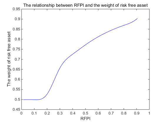
Figure 1.
The relationship between RFPI and the weight of risk-free asset
Figure 2
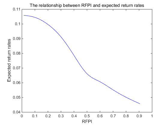
Figure 2.
The relationship between RFPI and expected return rates
Figure 3
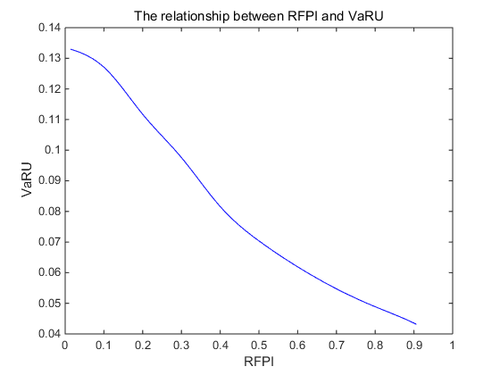
Figure 3.
The relationship between RFPI and VaRU
Figure 4
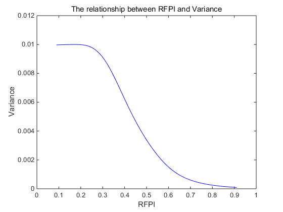
Figure 4.
The relationship between RFPI and variance
i) The weight of risk-free asset investments is positively related to RFPI.
As shown in Figure 1,the weight of risk-free asset investments increases rapidly as the RFPI value rises. When the RFPI value is 0.10, the weight of risk-free asset investments is 50%;when the RFPI value rises to 90%, the weight of risk-free assets increases to 88.90%. Therefore, investors should allocate more proportions to risk-free assets when choosing financial investments (e.g., endowment insurance investments).
ii) The expected return rate of a multi-objective uncertain portfolio is negatively correlated with RFPI.
As described in Figure 2, the expected return rate of a multi-objective uncertain portfolio decreases with an increase in RFPI. When the RFPI value is 0.10, the expected return rate of a multi-objective uncertain portfolio is 10.52%, which is far more than the risk-free return rate 4% (the preset value); when the RFPI value rises to 90%, the multi-objective uncertain portfolio’s expected return rate decreases to 4.60%. It can be seen that investors should take the potential risks into consideration when pursuing high returns, because the investment proportion of risk-free assets decreases and the protection effect is weaker at the same time.
iii) The VaRU of a multi-objective uncertain portfolio is negatively correlated with RFPI.
As depicted in Figure 3, the VaRU of a multi-objective uncertain portfolio decreases withan increase in RFPI. When the RFPI value is 0.10, the VaRU of a multi-objective uncertain portfolio is 12.96%; when the RFPI value rises to 90%, the VaRU of a multi-objective uncertain portfolio decreases to 4.40%. Thus, the restriction of a multi-objective uncertain portfolio to VaRU is stricter with a higher RFPI value. From Formulas (8) and (9), we find that the optimal VaRU is determined when the RFPI value is known in our proposed model (7) or model (10). Therefore, VaRU does not depend on the investors’ will or other subjective measurements.
iv) The variance of a multi-objective uncertain portfolio is negatively related to the RFPI value.
As portrayed in Figure 4, when the RFPI value is not greater than 0.03, the variance remains unchanged at 0.01; in other words, the portfolio risk corresponding to variance 0.01 can still satisfy the protection of possible future losses. When the RFPI value is greater than 0.03, the variance decreases with an increase in the RFPI value. It is easy to see that the limit value of the variance is 0.01 in model (14). Thus, risk conservatives who have their variance less than 0.01 can choose a RFPI value over 0.03, and they will obtain less expected returns. On the contrary, risk preferences often choose smaller RFPI values and receive higher expected returns. This conclusion is consistent with facts and intuition.
4.3. A Comparison Between the Multi-Objective Uncertain Portfolio Selection Model with FRPI Maximization and the MVM
Traditional and classical portfolio models (i.e., the mean-variance model) take the maximization of expected return as the objective function and variance as the risk constraint condition. Many scholars have studied portfolio problems based on MVM. Therefore, it is necessary, feasible, and effective to compare our RFPI model (7) with MVM when studying uncertain portfolio selection problems.
Using the data and assumptions of subsection 4.1, an uncertain portfolio without RFPI can be expressed as follows:
Thus, we can solve model (15), and the portfolio selections are shown in Table 5.
Table 5. Optimal portfolio selections based on MVM
| Stock 1 | Stock 2 | Stock 3 | Stock 4 | Bonds | Risk-free asset | Expected return rate | RFPI | Variance | VaRU |
|---|---|---|---|---|---|---|---|---|---|
| 0.0893 | 0.1380 | 0.1380 | 0.2281 | 0.0000 | 0.5000 | 0.1053 | 0.1020 | 0.0100 | 0.1328 |
| 0.0854 | 0.1092 | 0.1077 | 0.1455 | 0.0522 | 0.5000 | 0.0921 | 0.1913 | 0.0050 | 0.1098 |
| 0.0462 | 0.0500 | 0.0818 | 0.0515 | 0.1000 | 0.6705 | 0.0678 | 0.1913 | 0.0010 | 0.0784 |
Comparing the results of Tables 4 and 5 under the same level of risk-free assets weight, we find that theportfolio’s expected return is higher and the weight distribution of risk assets is more uniform and dispersed after RFPI maximization is added as the second objective function. Therefore, our proposed multi-objective uncertain portfolio model with FRPI maximization performs better than traditional MVM.
5. Conclusions
In order to further study the protective screening effect of a risk-free asset return on the risk assets and the portfolio selection expected returns, this paper followed the work of Gao and Liu [6] and proposed a RFPI model for a multi-objective portfolio with entropy and variance constraints based on the uncertainty theory. Compared with the model proposed by Gao and Liu [6], we maximized RFPI value under the premise of maximum expected return, and proportion entropy and variance constraints were also added to the FRPI model via the preset diversification requirement. Then, we found that the allocation proportion of risk assets is more uniform and dispersed and the portfolio’s expected return becomes greater after being added with an entropy constraint. Moreover, our proposed multi-objective uncertain portfolio model with FRPI maximization added as the second objective function performs better than traditional MVM.
In this paper, the authors assumed all security returns obey an independent and normal uncertain distribution. However, real markets are complicated and changeable, i.e., security returns are not completely subject to a normal uncertain distribution, and co-variance may exist in a pair of assets. In addition, we applied the widely-used Delphi method to estimate the uncertain expected return and standard deviation of different risk assets in our proposed models, but perhaps there are other methods that can be explored. Therefore, we can consider shedding light on multi-objective uncertain portfolio selections whose security returns satisfy an abnormal uncertain distribution or other kinds of distributions and new estimation methods in our future research.
Acknowledgements
This work was partly financially supported by the National Natural Science Foundation of China (No. 71671064) and the Fundamental Research Funds for the Central Universities (No. 2018ZD14, 2016XS70).
Reference
Risk Index based Models for Portfolio Adjusting Problem with Returns Subject to Experts' Evaluations
,”
DOI:10.1016/j.econmod.2012.09.032
URL
[Cited within: 2]

This paper discusses a portfolio adjusting problem with additional risk assets and a riskless asset in the situation where security returns are given by experts' evaluations rather than historical data. Uncertain variables are employed to describe the security returns. Using expected value and risk index as measurements of portfolio return and risk respectively, we propose two portfolio optimization models for an existing portfolio in two cases, taking minimum transaction lot, transaction cost, and lower and upper bound constraints into account. In one case the riskless asset can be both borrowed and lent freely, and in another case the riskless asset can only be lent and the borrowing of riskless asset is not allowed. The adjusting models are converted into their crisp equivalents, enabling the users to solve them with currently available programming solvers. For the sake of illustration, numerical examples in two cases are also provided. The results show that under the same predetermined maximum tolerable risk level the expected return of the optimal portfolio is smaller when the riskless asset can only be lent than when the riskless asset can be both borrowed and lent freely. (c) 2012 Elsevier B.V. All rights reserved.
A Risk Index Model for Portfolio Selection with Returns Subject to Experts' Estimations
,”
DOI:10.1007/s10700-012-9125-x
URL
[Cited within: 6]
AbstractPortfolio selection is concerned with selecting an optimal portfolio that can strike a balance between maximizing the return and minimizing the risk among a large number of securities. Traditionally, security returns were regarded as random variables. However, there are cases that the predictions of security returns are given mainly based on experts judgements and estimations rather than historical data. In this paper, we introduce a new type of variable to reflect the subjective estimations of the security returns. A risk index for uncertain portfolio selection is proposed and a new safe criterion for judging the portfolio investment is introduced. Based on the proposed risk index, a new mean-risk index model is developed and its crisp forms are given. In addition, to illustrate the application of the model, two numerical examples are also presented.
A Risk Index Model for Multi-Period Uncertain Portfolio Selection
,”
DOI:10.1016/j.ins.2012.06.017
URL
[Cited within: 5]
This paper discusses a multi-period portfolio selection problem when security returns are given by experts’ evaluations. The security return rates are regarded as uncertain variables and an uncertain risk index adjustment model is proposed. Optimal portfolio adjustments are determined with the objective of maximizing the total incremental wealth within the constraints of controlling the cumulative risk index value over the investment horizon and satisfying self-financing at each period. To enable the users to solve the model problem with currently available programming tools, an equivalent of the model is provided. In addition, a method of obtaining the uncertainty distributions of the security returns is given based on experts’ evaluations, and a selection example is presented.
A Risk-Free Protection Index Model for Portfolio Selection with Entropy Constraint under an Uncertainty Framework
,”
Delphi Method for Estimating Uncertainty Distributions
,”
Mean-Chance Model for Portfolio Selection based on Uncertain Measure
,”
DOI:10.1016/j.insmatheco.2014.10.001
URL
[Cited within: 1]
This paper discusses a portfolio selection problem in which security returns are given by experts’ evaluations instead of historical data. A factor method for evaluating security returns based on experts’ judgment is proposed and a mean-chance model for optimal portfolio selection is developed taking transaction costs and investors’ preference on diversification and investment limitations on certain securities into account. The factor method of evaluation can make good use of experts’ knowledge on the effects of economic environment and the companies’ unique characteristics on security returns and incorporate the contemporary relationship of security returns in the portfolio. The use of chance of portfolio return failing to reach the threshold can help investors easily tell their tolerance toward risk and thus facilitate a decision making. To solve the proposed nonlinear programming problem, a genetic algorithm is provided. To illustrate the application of the proposed method, a numerical example is also presented.
Mean-Variance Models for Portfolio Selection Subject to Experts' Estimations
,”
DOI:10.1016/j.eswa.2011.11.119
URL
[Cited within: 1]
Since the security market is complex, sometimes the future security returns are available mainly based on experts judgements. This paper discusses a portfolio selection problem in which security returns are given subject to experts’ estimations. The use of uncertain measure is justified, and two new mean–variance and mean–semivariance models are proposed. In addition, a hybrid intelligent algorithm for solving the optimization models is given. To illustrate the application of the new models, the method to obtain the uncertainty distributions of the security returns based on experts’ evaluations is given, and two selection examples are provided.
