


1. Introduction
For software product acceptance, we test whether the software reliability index reaches the standard through software reliability demonstration testing [1]. In general, the higher the confidence coefficient of demonstration results, the better the reliability of software, but the workload of testers is also greatly increased. Especially for some software products with complex technology, the economic cost, labor cost, and time cost of acceptance are unacceptable, making software reliability demonstration testing difficult to complete. However, a Bayesian method can effectively utilize prior information and can significantly reduce the workload of reliability demonstration testing under the condition of ensuring a high confidence coefficient.
At present, experts and scholars have conducted a lot of research on software reliability demonstration testing of the Bayesian method. Tan applied a Bayesian method of constructing a conjugate distribution to verify software reliability [2]. Then, he continued to propose a reliability demonstration testing method based on prior dynamic integration [3]. Liu proposed a weighted Bayesian method based on multi-stage prior information [4]. By constructing a hybrid prior distribution, Zhang gave a reliability demonstration testing scheme under the condition of hybrid prior distribution. [5] Wang put forward a reliability demonstration testing scheme based on the prior distribution method with a decreasing function [6]. Liu proposed a multi-layer Bayesian software reliability demonstration testing method based on a decreasing function [7].
All of these methods are based on ideal and simple conditions [8-10]. For example, supposing the number of estimated parameters is reduced to one in the prior distribution function, the prior distribution function of a multi-layer Bayesian has uniform distribution. Additionally, prior dynamic integration considers the situation of zero-failure demonstration testing and does not consider the situation of non-zero-failure. Therefore, the results of previous studies exhibit one-sidedness and are also not suitable for universal software reliability demonstration testing. Therefore, this article makes further research on the basis of previous studies. Firstly, a prior distribution function of two parameters with a monotone decreasing function is constructed. Secondly, a software reliability demonstration testing scheme of a Bayesian method based on the monotone decreasing function is proposed. At the same time, a specific parameters estimation method is given. Thirdly, two kinds of prior dynamic integration methods are proposed to deal with the different failure times in the actual testing process. Finally, through experimental analysis, it is illustrated that the demonstration scheme can reduce the testing duration and the two kinds of prior dynamic integration methods are feasible.
2. Basic Principle of Bayesian Theory of Reliability Demonstration Testing
In the process of reliability demonstration testing [11-12], the failure rate $\lambda$ is selected as the reliability index, and the conditional distribution density function of the failure times is $f(r\left| \lambda \right.)$. At the same time, $h(\lambda )$ is the prior distribution density function of$\lambda $. Then, the joint distribution density function of the failure times and the failure rate is as follows:
UsingFormula (1), the edge distribution of the failure times is obtained:
The combination of Formula (1) and Formula(2) is used to further deduce the posterior distribution density function of the failure rate, namely:
According to the actual situation, the reliability index (${{\lambda }_{0}},r,c$) is set up in the reliability demonstration testing scheme. Among them: the failure times is r, the failure rate is ${{\lambda }_{0}}$, and the confidence coefficient is c. We solve the t of the minimum value, which is the shortest total testing time for the reliability demonstration testing scheme.
3. Bayesian Software Reliability Testing Scheme based on the Idea of Monotone Decreasing Function
3.1. Determination of the Prior Distribution and the Posteriori Distribution
In order to construct a prior distribution function with a monotone decreasing function, the kernel of the function is explained. Suppose $f(x)$ is the distribution density function of a random variable. If $f(x)={A}'g(x)$, ${A}'$ is a polynomial that has nothing to do with random variables and $g(x)$ is a polynomial containing all the random variables. Then, $g(x)$ is the kernel of the $f(x)$ function, namely:
According to the idea of decreasing functions, we regard the failure rate $\lambda$ as the random variable of a gamma distribution, and we construct the kernel of the distribution density function of a monotone decreasing function, that is:
Among them: a and b are parameters to be estimated, $0<a\le 1,\text{ }b>0$.
Using the concept of the kernel of the function, we can get the prior distribution density function of $\lambda$, that is:
The Bayesian software reliability demonstration testing scheme selects the failure rate of the prior distribution density function, which is to satisfy the gamma distribution. For convenience of computing, $h(\lambda )$ is slightly changed, namely, ${A}'\text{=}A{{b}^{a-1}}$. Then, the prior distribution density function $h(\lambda)$ based on the idea of decreasing functionsis changed to:
According to the property of the distribution density function, we can get the following:
Then, we can get $A=b/\Gamma (a)$ and deduce the density function of $\lambda$ prior distribution, that is:
Among them: $\Gamma (a)$ is a gamma function, and its expression is: $\Gamma (a)=\int_{0}^{+\infty }{{{s}^{a-1}}{{e}^{-s}}\text{d}s},\text{ }a>0$.
It is assumed that the probability of failure times ($X=r$) is the conditional probability of $\lambda $in the time interval$\left( 0 \right.,\left. t \right]$. Failure times obey the $\lambda t$ Poisson distribution, that is:
Joining Formula (10) and Formula (11), we can get the joint distribution function of $X,\text{ }\lambda $, that is:
From the upper formula, we can deduce the edge distribution function of X, that is:
Joining Formula (12) and Formula (13), the posterior distribution density function $\lambda$ can be obtained, that is:
3.2. Solving Parameters’ Values
In the prior distribution density function $h(\lambda)$, parameters a and bare estimated according to the obtained relevant information in the software reliability testing phase [13-14]. We can determine the estimated values of parameters using the software reliability testing total time t and the expectation and variance of failure times.
The software reliability testing total time t is assumed to be long enough. We divide time interval $\left( 0 \right.,\left. t \right]$ into m time interval sequences ${{T}_{1}},{{T}_{2}},\cdots ,{{T}_{m}}$. Then, failure times is${{k}_{i}}{=t}/{{{T}_{i}}}\;,\text{ }(i=1,2,\cdots ,m)$ in each time interval${{T}_{i}}$.
The edge distribution function of $p(r)$ corresponding to the first moment:
The edge distribution function of $p(r)$ corresponding to the second moment:
$E(r)$ and $E({{r}^{2}})$are recorded as ${{w}_{1}},\text{ }{{w}_{2}}$. The estimated values of parametersa, b are:
Among them: $\text{Among}\ \text{them}:\ {{w}_{1}}=\frac{1}{m}\sum\limits_{i=1}^{m}{{{k}_{i}}},\text{ }{{w}_{2}}=\frac{1}{m}\sum\limits_{i=1}^{m}{k_{i}^{2}}$
3.3. Software Reliability Demonstration Testing Scheme
According to the basic principle of the Bayesian reliability testing method[15], the software reliability demonstration testing scheme of the Bayesian method based on a monotone decreasing function is formulated, namely:
4. Prior Dynamic Integration
If the software is tested in the specified reliability demonstration testing time[16], the actual total failure times is not greater than the maximum failure times. Then, we stop testing and receive this testing software; otherwise, the next software reliability demonstration testing is required to be continuous. Obviously, the experience of previous testing failure certainly provides historical information for the next reliability demonstration testing. Therefore, we should merge the result information of the last testing failure with prior information of the next software reliability demonstration testing.
4.1. Prior Dynamic Integration Method under the Condition of Error Correction
Generally speaking, for safety critical software, high reliability software, aerospace software, and other types of software, when a defect that causes failure is found during software reliability demonstration testing, it should be misarranged immediately; this is conducive to improve the reliability of the software itself. At the same time, for the high reliability software, the test conditions are more stringent, so we generally choose zero-failure testing. Aiming at the above two points, this paper puts forward a prior dynamic integration method under the condition of error correction.
If the software actual testing length ${{{t}'}_{1}}$ does not exceed t1and ${{r}_{1}}=r+1$, then the software reliability does not meet the reliability standard. At the moment, we should immediately stop the testing and correct the error, and then continue reliability demonstration testing. Obviously, when the software performs the first reliability demonstration testing, the failure times is greater than the maximum failure times at moment ${{{t}'}_{1}}$. The different moment of occurrence gives us different information. Therefore, when performing the next reliability demonstration testing, the result information of the last testing failure needs to be merged with prior information of the next software reliability demonstration testing. Then, software testing duration t2 should satisfy the following formula t:
It can be followed by analogy. When the (i-1)th reliability demonstration testing does not pass, then the corresponding testing length tiof the ith demonstration testing should satisfy following formula t:
Through the above analysis, the following gives a prior dynamic integration method under the condition of error correction. The specific process is as follows:
The first step: According to formulating the software reliability demonstration testing scheme of a Bayesian method based on a monotone decreasing function and reliability index $({{\lambda }_{0}},r,c)$, we use Formula(18) to calculate the testing duration t.
The second step: In the testing duration t, if ${{r}_{i}}\le r$ and the demonstration testing is passed, then the software is received and testing is over; otherwise, proceed to the third step.
The third step: The longest testing duration that the tester can accept is tmax, the maximum number of iterations is I, and the number of initial iterations is one, namely $i=1$.
The fourth step: Let the actual total testing duration time ${{t}_{all}}=\sum\limits_{i=1}^{i-1}{{{{{t}'}}_{i}}+{{t}_{i}}}$ and $i=i+1$. According to Formula (20), we calculate the testing duration ti under the condition of reliability indicators $({{\lambda }_{0}},r,c)$. If ${{r}_{i}}\le r$,the demonstration testing passes, the software is received, and testing ends; otherwise, judge whether the demonstration testing is over and calculate total actual testing duration ${{t}_{all}}$ at the moment. If ${{t}_{all}}>{{t}_{\max }}$ or $i>I$, the testing ends, the acceptance fails, and the software is rejected. Otherwise, we find the moment ${{{t}'}_{i}}$ of the actual failure times ${{r}_{ac}}=r+1$ in the testing process and then continue to repeat the fourth step.
4.2. Prior Dynamic Integration Method Without Correction Error
Analogous to the error correction prior dynamic integration method, a reliability demonstration testing that does not consider zero-failure testing is proposed. The method is aimed at software that fails at least once in the actual testing process, that is, $r\ne 0$. The following introduces a prior dynamic integration method without correction error.
The first step: According to formulating a software reliability demonstration testing scheme of a Bayesian method based on a monotone decreasing function and reliability index $({{\lambda }_{0}},r,c)$, we use Formula(18) to calculate the testing duration t.
The second step: In the testing duration t, if ${{r}_{i}}\le r$ and demonstration testing is passed, then the software is received and testing is over; otherwise, proceed to the third step.
The third step: Thelongest testing duration that the tester can accept is tmax, the maximum number of iterations is I, and the number of initial iterations is one, namely $i=1$.
The fourth step: Let ${{r}^{*}}=(\left\lceil \frac{r{}_{i}-r}{r} \right\rceil +1)r$(as shown in the formula, r must not be 0, which means that this method is not suitable for zero-failure software reliability demonstration testing). Substituting failure times ${{r}^{*}}$ into Formula (18) during the actual testing process, the total testing duration t*is calculated under the reliability index (a, b, c). If ${{t}^{*}}>{{t}_{\max }}$ or $i>I$, the testing is over, the acceptance is not passed, and the software is rejected; otherwise, we proceed to the fifth step.
The fifth step: We continue software reliability demonstration testing during (${{t}^{*}}-t$) hours. If failure times is not greater than (${{r}^{*}}-{{r}_{i}}$), the validation passes, the software is received, and the testing is finished; otherwise, we proceed to the sixth step.
The sixth step: Supposing there are k failures in the(${{t}^{*}}$)-t testing duration, then let ${{r}_{i+1}}={{r}_{i}}+k,\text{ }t={{t}^{*}}$ and $i=i+1$, and then we repeat the fourth step.
4.3. Prior Dynamic Integration Method under Two Conditions
According to the above two kinds of situations, through the combination of the two methods, a prior dynamic integration method under two different conditions is proposed. The flowchart is shown in Figure 1, and detailed steps are as follows:
Figure 1
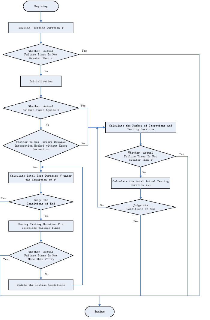
Figure 1.
The specific flow chart of priordynamic integration method
The first step: According to the software reliability demonstration testing scheme of a Bayesian method based on a monotone decreasing function, we use Formula(18) to calculate the testing duration. In the process of testing, if ${{r}_{ac}}\le r$, then software passes reliability demonstration testing; otherwise, we take the second step.
The second step: Thelongest testing duration that the tester can accept is tmax, the maximum number of iterations is I, and the number of initial iterations is one, namely $i=1$.
The third step: According to the actual requirements of testing, we determine whether the reliability demonstration testing is zero-failure demonstration testing. If there is zero-failure demonstration testing, then the prior dynamic integration method under the condition of error correction is chosen. The specific process refers to Section 4.1; otherwise, proceed to the fourth step.
The fourth step: In the case of non zero-failure times, we can choose either of the two methods. If we choose the priordynamic integration method without correction error, then the specific steps refer to Section 4.2. Otherwise, refer to Section 4.1.
5. Experimental Analysis
5.1. Experimental Results
In this paper, the time-controlled software that is developed by our laboratory is selected. The prior information of the experiment comes from the special vehicle software evaluation centre. During the process of software reliability growth, the failure interval data of the last 10 sets is obtained and constitutes historical information. Selecting t=100000 hours, we obtain the empirical sample values $t/{{T}_{i}}$ of failure times at this stage, which constitute prior information data, as shown in Table 1.
Table 1. Prior information data
| Failure interval time | Failure times |
|---|---|
| 1136.36 | 88 |
| 649.35 | 154 |
| 7142.86 | 14 |
| 396.83 | 252 |
| 943.40 | 106 |
| 8333.33 | 12 |
| 335.57 | 298 |
| 2173.91 | 46 |
| 16666.67 | 6 |
| 5555.56 | 18 |
Through prior information data, combining with Formula (17), we can get the estimated value of the prior distribution parameter of failure rate.
The values of $a=1,\text{ }b=1008$ are consistent with the range of parameter values of the prior distribution function based on a monotone decreasing function, then $h(\lambda )=1008{{e}^{-1008\lambda }}$. In the demonstration testing scheme, the confidence coefficient c is 0.99, failure rate ${{\lambda }_{0}}$ is 0.001, and failure times r are from 0 to 10. Using Formula (18), we get the total time length of software reliability demonstration testing under the condition of no prior information and prior information with a monotone decreasing function. The results are shown in Table 2.
Table 2. Total testing durationbased on different prior information
| Failure times | No prior information | Prior information with monotone decreasing function |
|---|---|---|
| 0 | 4601 | 3593 |
| 1 | 6633 | 5625 |
| 2 | 8400 | 7392 |
| 3 | 10039 | 9031 |
| 4 | 11598 | 10590 |
| 5 | 13100 | 12092 |
| 6 | 14563 | 13555 |
| 7 | 15992 | 14984 |
| 8 | 17395 | 16387 |
| 9 | 18775 | 17767 |
According to the prior dynamic integration method under the conditions of no prior information and prior information with a monotone decreasing function and with the conditions of failure times respectively from 0 to 3, the relationship between the actual failure times and the total demonstration testing duration is shown in Tables 3-6 during the software reliability demonstration testing.
Table 3. r = 0, the result diagram of total testing duration
| Actual failure times | The total testing duration under the condition of error correction |
|---|---|
| 0 | 3593 |
| 1 | 5625 |
| 2 | 7392 |
| 3 | 9031 |
| 4 | 10590 |
| 5 | 12092 |
| 6 | 13555 |
| 7 | 14984 |
Table 4. r = 1, the result diagram of total testing duration
| Actual failure times | The total testing duration under the condition of error correction | The total testing duration without correction error |
|---|---|---|
| 0 | 5625 | |
| 1 | ||
| 2 | 9031 | 7392 |
| 3 | 9031 | |
| 4 | 12092 | 10590 |
| 5 | 12092 | |
| 6 | 14984 | 13555 |
| 7 | 14984 | |
Table 5. r = 2, the result diagram of total testing duration
| Actual failure times | The total testing duration under the condition of error correction | The total testing duration without correction error |
|---|---|---|
| 0 | 7392 | |
| 1 | ||
| 2 | ||
| 3 | 12092 | 10590 |
| 4 | ||
| 5 | 13555 | |
| 6 | 16387 | |
| 7 | 16387 | |
Table 6. r = 3, the result diagram of total testing duration
| Actual failure times | The total testing duration under the condition of error correction | The total testing duration without correction error |
|---|---|---|
| 0 | 9031 | |
| 1 | ||
| 2 | ||
| 3 | ||
| 4 | 14984 | 13555 |
| 5 | ||
| 6 | ||
| 7 | 17767 | |
5.2. Results Analysis
According to Table 2, the following three related conclusions can be obtained:
1) First of all, with an increase in failure times, the testing duration increases regardless of whether there is prior information or not. Secondly, it can be found that with an increase in failure times, the growth rate of testing duration decreases. For example, in the demonstration testing scheme without prior information, when failure times increase from 0 to 1, the growth rate of testing duration is 44.2%. When failure times increase from 9 to 10, the growth rate of testing duration is 5.3%. In the Bayesian demonstration testing scheme based on the monotone decreasing function, the growth rate of testing duration is 56.6% when failure times increase from 0 to 1. The growth rate of testing duration is 7.7% when failure times increase from 9 to 10.
2) Obviously, in the Bayesian demonstration scheme based on the monotone decreasing function, the testing duration is significantly less than the testing duration without prior information testing scheme. When failure times is 0, the testing duration of the proposed testing scheme is shortened by 28.1% compared with the testing duration without prior information. When the failure number is 10, the testing duration of the proposed testing scheme is shortened by 5.3% compared with the testing duration without prior information.
3) As failure times increases, the testing duration becomes closer and closer between the two schemes. This shows that if software reliability is not high, the software will be very prone to failure in software reliability demonstration testing. If the condition of receiving software corresponding to failure times is too large, no matter which testing scheme is used, this will bring tremendous workload to testers and expend a large amount of time, possibly even making it impossible to complete the software reliability demonstration testing.
According to Tables 3-6, the following three related conclusions can be obtained:
1) Aiming at different failure times, when the actual cumulative failure times is in single digits during the demonstration testing, the testing duration of the prior dynamic integration method without error correction is no longer than the prior dynamic integration method with error correction. For example, when $r=1$ and the actual cumulative failure times is 2, the testing duration of the prior dynamic integration method without error correction is reduced by 1639 hours compared with that of the prior dynamic integration method with error correction. However, when $r=1$ and the actual cumulative failure times is 5, the prior dynamic integration method without error correction has the same testing duration as the prior dynamic integration method with error correction.
When the actual cumulative failure times is too large in the process of demonstration testing, the testing duration of the prior dynamic integration method with error correction is shorter than that of the prior dynamic integration method without error correction. With the continuous increase in actual cumulative failure times, the testing duration of the prior dynamic integration method with error correction is obviously smaller than that of the prior dynamic integration method without error correction. For example, when $r=3$ and the actual cumulative failure times is 7, the testing duration of the prior dynamic integration method with error correction is shortened by 2784 hours compared with that of the prior dynamic integration method without error correction. This shows that when software cumulative failure times frequently increase, if the defect is not corrected, then the prior dynamic integration method without error correction will waste more testing time. The testing duration will even exceed the controllable range of testers, meaning that software reliability demonstration testing cannotbe completed. Therefore, in order to avoid such events, failures will be corrected in real time during the testing process, and then the next software reliability demonstration testing will be continued.
2) Analysis of the prior dynamic integration method under the condition of error correction: Because all the demonstration testing results are similar, select the number of failure times as 1 to analyse in the testing scheme. When the software performs the first reliability demonstration testing, the testing duration is 5625 hours. During this period, if software failure times is no more than 1, then the software is accepted, the reliability indicator is up to standard, and the software is received. If the value of failure times is two at ${{{t}'}_{1}}=3000$ hours (${{{t}'}_{1}}<{{t}_{1}}$), then the software acceptance fails andthe reliability does not reach the standard. In this case, we need to stop the demonstration testing, immediately correct the software default, and then continue with the second demonstration testing. The second testing duration is ${{t}_{2}}=5625-{{{t}'}_{1}}=2625$ hours. Similarly, in the first demonstration testing process, if the value of failure times is two at ${{{t}'}_{1}}=4200$ hours, then the software acceptance fails andthe reliability indicators do not meet the standard. Namely, the second testing duration is ${{t}_{2}}=5625-{{{t}'}_{1}}=1425$ hours. It is obvious that the time point that is not passed through the first demonstration testing has a direct impact on the duration of the second demonstration testing. If we proceed with the second demonstration testing and the value of failure times is two at the moment ${{{t}'}_{2}}$, then the software acceptance is not passed andthe reliability is not up to the standard. We need to perform the third reliability demonstration testing for software, and the third testing duration is ${{t}_{3}}=9031-{{{t}'}_{2}}$$-{{{t}'}_{1}}$ hours. It can be seen that the third testing duration is related to the previous two time points that are not passed through the demonstration testing, which indicates that the previous two demonstration testing results have an impact on the third testing duration. Therefore, in the course of the next software reliability demonstration testing, all of the preceding demonstration testing results (testing duration) need to be integrated and analysed. The analysis of the following testing results is analogous in turn.
3) Analysis of the prior dynamic integration method without error correction:Because all the demonstration testing results are similar, select the number of failure times as 2 to analyse in the testing scheme. When the software performs the first reliability demonstration testing, the testing duration is 7392 hours. During this period, if software failure times is no more than 2, then the software is accepted, the reliability indicator is up to standard, and the software is received. If ${{r}_{1}}=4$, (${{r}_{1}}>r$) at the end of the testing, then the software acceptance fails and the reliability is not up to standard. At the moment, we do not need to troubleshoot, but instead follow the second demonstration testing. The second demonstration testing duration is $t={{t}^{*}}-t=10590-7932$$-\text{3198}$ hours. Similarly, if ${{r}_{1}}=5$ in the process of the first testing, then the reliability indicator did not meet the standard. Namely, the second testing duration is $t={{t}^{*}}-t$$=13555-7392=6163$. After the first demonstration testing, it can also be obtained that the actual cumulative failure times have a direct impact on the duration of the second demonstration testing. If we proceed with the second demonstration testing and ${{r}_{2}}>r$, then the software acceptance is not passed andthe reliability is not up to standard. We need to perform the third reliability demonstration testing for the software, and the third testing duration equals this testing duration minus the last testing duration. Therefore, over the course of the next software reliability demonstration testing, all of the preceding demonstration testing results (cumulative failure times) need to be integrated and analysed. The analysis of the following testing results is analogous in turn.
6. Conclusions
In this paper, a reliability demonstration testing scheme based on a Bayesian method is introduced. Then, the prior distribution function with a monotone decreasing function is proposed, and the prior distribution based on a monotone decreasing function and the corresponding posterior distribution are established. Then, the estimation method of parameters is given in prior distribution. On the basis of this, a software reliability demonstration testing scheme of a Bayesian method based on a monotone decreasing function is proposed. Then, prior dynamic integration methods under two different conditions are proposed. One of them is a prior dynamic integration method under the condition of error correction, which mainly integrates prior information of testing duration; the other is a prior dynamic integration method without error correction, which mainly integrates prior information of failure times.
Through experimental analysis, compared with the demonstration testing scheme without prior information, this scheme can significantly reduce demonstration testing duration of software reliability and ensuresoftware reliability demonstration testing resultsunder the same confidence condition. At the same time, the prior dynamic integration method makes comprehensiveconsideration of the real-time dynamic prior information of testing software during the process of software reliability demonstration testing, which effectively reduces the testing duration of reliability demonstration.
Of course, the software reliability demonstration testing scheme of a Bayesian method based on a monotone decreasing function still needs to be invested in many demonstration testing experiments, so as to continuously improve this method. Then, it will be more efficient to apply this method to software reliability demonstration testing.
Reference
Software Reliability Validation and Verification Using Fault Injection Techniques on a Fault TolerantProcessor
,”
DOI:10.1016/j.ifacol.2015.08.140
URL
[Cited within: 1]

Due to the continuously increasing complexities of embedded electronic systems, there is a clear need for more sophisticated methods of testing and evaluating the performances and reliabilities of the embedded software. One such method is to simulate potentially dangerous events, while monitoring the system's response and stability. This paper presents a software simulation tool, which will be used for evaluating the mission critical software of the TRISAT mission. The software simulation tool simulates, on a per-cycle basis, the fault tolerant processor and its peripherals while also simulating the effects of the space environment on the simulated hardware. Using the simulation software, a dependability analysis was performed regarding the use of Error Correction and Detection Codes on the processor data memory as well as the rate of memory scrubbing, using two benchmark algorithms: matrix multiplication and quick sort.
Research on Reliability Demonstration Testing of Safety CriticalSoftware
,”
Software Reliability Demonstration Testing Plan based on Bayesian Theory
,”
DOI:10.4028/www.scientific.net/AMR.658.513
URL
[Cited within: 1]

For highly reliable software, it is expensive, time consuming or even infeasible to perform reliability testing by traditional Bayesian-based software reliability demonstration testing plan. Meanwhile, when determining the prior distribution function, people only consider conjugate prior distribution in order to realize the calculation in mathematics but ignores the characteristics of highly reliable software. To address this problem, by introducing the construction method of multilayer prior distribution function into the software reliability demonstration testing plan, this paper put forward a new Bayesian software reliability demonstration testing plan with zero-failure data, which can be used for highly reliable software reliability demonstration testing. Finally through examples, it illustrated the superiority of the method.
Weighted Bayesian Method of Reliability Evaluation for Binomial Product
,”
DOI:10.3969/j.issn.1004-132X.2013.24.021
URL
[Cited within: 1]
Because of defects of classical statistical method and traditional Bayesian method,a reliability evaluation method of binomial products based on the multi- stage information was proposed. The concept of similarity coefficient was introduced based on the chi-square goodness of fit. The similarity coefficients of each stage is got test information and field test information were determined respectively. Then the confidence lower limit was determined with each stage is got test information as information prior to the field test. Finally,the confidence lower limit of the product. The simulation examples show that the calculation results are between classical statistical method and traditional Bayesian method,and the evaluation result is more reasonable.
Multiple-Layer Bayesian Discrete Software Reliability Demonstration Testing Scheme with Decreasing Function
,”For decreasing the required testing effort of software reliability demonstration testing( SRDT),and meeting the demonstration requirement of software with high-reliability,this paper proposed a multiple-layer Bayesian reliability demonstration testing scheme with decreasing function for the discrete software( MBDFDSRDT) based on the Bayesian theory and the decreasing function. First,it selected the decreasing function of failure probability as the prior distribution function of the first layer. And then it used hyper-parameters to construct the prior distribution function of the second layer. Furthermore,it proposed the multiple-layer poster distribution function based on the prior functions of the first and second layers. Finally,it applied the proposed MBDFDSRDT on several failure data-sets. The experiment results illustrate that compared with the Bayesian-SRDT and the single-layer Bayesian discrete SRDT,the proposed MBDFDSRDT in this paper is more effective and applicable for significantly decreasing the required testing effort of SRDT especially for the critical software with high reliability.
Analysis of Correlation Coefficient Influence on Software Reliability Demonstration Testing
,”In the process of software reliability demonstration testing there is a problem that traditional Bayesian method did not distinguish between historical information and experimental information.A hybrid Bayesian software reliability demonstration testing scheme is proposed.By introducing the concept of correlation coefficient,the correlation coefficients in hybrid Beta distribution are determined by subjective quantitative method,goodness of fit method,Kullback information method,Spearman correlation coefficient method and Kendall correlation coefficient method respectively.Finally,through experimental analysis,prove the feasibility of the 5 kinds of calculation method of correlation coefficient,and prove that differentiating the historical information and experimental information impacts acceptable quality level of software reliability demonstration testing.
Reliability Demonstration Testing Method for Continuous Execution Software
,”
Study on the Reliability Demonstration Testing Method for Safety-Critical Software
,”
Planning Reliability Demonstration Test with Performance Requirements
” in
DOI:10.1109/RAM.2017.7889733
URL
Carefully planning reliability testing is necessary for success of a product development. Sample size determination is an important step in test planning. One of most common questions any reliability engineer gets asked is ow many units do we need to test? Of course the answer depends on a number of factors and information in hand. The design of reliability demonstration testing (RDT) has been widely studied by many researchers. Most planning methods are based on the time-to-failure properties of product under test, such as the Binomial equation, the Chi-Squared formula, and etc. However, quite often, reliability test requirements are defined by certain performance characteristic(s), or physical characteristic(s), or quality characteristic(s). Very few works have been published to plan a reliability test with performance measurements directly. Some works on degradation measurements analysis, including degradation test plan for Wiener degradation processes, have been carried out for maintenance optimization purpose. This paper develops a test planning method for reliability demonstration test when the reliability test requirement is constructed with its performance or degradation measurements. A simple formula for sample size determination is provided in the paper, and a couple of case studies will be presented to help reliability practitioners to plan the reliability testing using the proposed method.
Continues Software Reliability Demonstration Testing Scheme with Decreasing Function
,”The required testing duration of software reliability demonstration testing(SRDT) for the continuous safety-critical software is generally too long to endure.To solve this problem,a new continuous Bayesian-based SRDT scheme(CBSDF) for the safety-critical software is proposed by using the decreasing function method with the prior information.The representative decreasing function of the continuous reliability index(such as the failure rate) is selected to construct the prior distribution density function(PDDF).Then,the estimation values of the hyper-parameters of PDDF are calculated according to the prior information(i.e.the failure data collected in reliability growth testing) to obtain the posterior distribution and the detailed form of CBSDF.By selecting two failure data-sets as the source of prior information,the proposed CBSDF is compared with two existing Bayesian-based schemes(i.e.CBS1 without prior information and CBS2 with prior information).The experimental results show that with the same given reliability index,the proposed CBSDF is more effective than CBS1 and CBS2 by significantly decreasing the required testing time of SRDT and more suitable for the safety-critical software with high reliability.
Method for Testability Demonstration Test Design based on Entropy of Prior Test Information
,”In the development stage,there is a large number of test data.Aiming to making good use of the prior test data and reducing the sample number of testability demonstration test,a method for testability demonstration test design based on information entropy of prior test information is proposed.In the method information entropy is used to check the role of different prior test data for the testability demonstration test,and many times prior test data is equivalent to success or failure data at a time according to the principles of equal mean interactive entropy and equal total information.On this basis,compatibility of prior data and test data is established by the method of compatibility test,while Beta distribution is made use as prior distribution and the mixed posteriori distribution is established by weighted hybrid Bayesian theory.Then,testing scheme satisfying the risk requirement of producer and consumer is solved based on Bayesian average risk theory.At last,to verify the proposed method,an example of a certain type of transmitter is given,and the result shows the validity of the proposed method.
Design of Safety-Critical Software Reliability Demonstration Test based on Bayesian Theory
,” in
DOI:10.1109/QR2MSE.2013.6625734
URL
[Cited within: 1]
The original software reliability demonstration test (SRDT) takes no consideration of prior knowledge and priori distribution adequately, which costs a lot of time and resource. A new improved Bayesian based SRDT method was proposed. First, a framework for SRDT scheme was constructed. According to the framework the decreasing function was employed to construct the priori distribution density functions for discrete and continuous safety-critical software respectively, and then discrete Bayesian software demonstration function (DBSDF) scheme and continuous Bayesian software demonstration function (CBSDF) scheme were presented. A set of comparative experiments have been carried out with the classic demonstration testing scheme on several published data sets. The experimental results reveal that both DBSDF scheme and CBSDF scheme are more efficient and applicable especially for the safety-critical software with high reliability requirements.
Bayesian Theory based Software Reliability Demonstration Test Method for Safety Critical Software
,”
DOI:10.1017/S0960129513000789
URL
[Cited within: 1]
The original software reliability demonstration test (SRDT) does not take adequate account of prior knowledge or the prior distribution, which can lead to an expensive use of many resources. In the current paper, we propose a new improved Bayesian based SRDT method. We begin by constructing a framework for the SRDT scheme, then we use decreasing functions to construct the prior distribution density functions for both discrete and continuous safety-critical software, and then present schemes for both discrete and continuous Bayesian software demonstration functions (which we call DBSDF and CBSDF, respectively). We have carried out a set of experiments comparing our new schemes with the classic demonstration testing scheme on several published data sets. The results reveal that the DBSDF and CBSDF schemes are both more efficient and more applicable, and this is especially the case for safety-critical software with high reliability requirements.
Analysis on Software Reliability Testing Technology
”
A New Hierarchical Testing Model in Software Reliability Testing
,”in
Reliability Assessment for Device with Only Safe-or-Failure Pattern based on Bayesian HybridPrior Approach
,”For the reliability evaluation of device with only safe-or-failure pattern,a hyprid prior approach is introduced,and the posteriori probability distribution function of reliability parameter is deduced by Bayesian method. The influence of prior distribution parameters on the posterior estimation is considered,and the general rules of choosing these parameters are summarized. The parameter posterior estimates of traditional Bayesian method and hyprid prior approach are compared. The results indicate that the hyprid prior approach can avoid the problem of that the prior data inundate the posteriori data effectively. The analysis of posteriori mean square error demonstrates that the hyprid prior approach can improve the performance of estimation to some extent. Through the comparison with power prior approach,it is proved that the estimation effect of hyprid prior approach is better than that of power prior approach,especially when prior sample size is larger.
