


1. Introduction
Risk-based maintenance is widely used in high-risk areas such as aerospace. With the upgrading of equipment systems, the design of related systems has become more and more complicated, and some kinds of risks that may arise in equipment systems have also become more and more diversified. Due to the poor operating environment, the maintenance becomes complicated and difficult. Any problems in the design, manufacture and maintenance of the products may cause some economic losses as well as serious safety accidents. Therefore, it is necessary to analyze the safety risk of related systems and make scientific and effective maintenance decisions during operation or storage. It is of vital significance to aerospace products to control the risk within a certain range.
Although there are several definitions for risk, in maintenance engineering it has always been viewed as a combination of two attributes: likelihood (i.e., a description, even rough, of the uncertainty in the occurrence of the failure event) and severity (i.e., a quantification of the impact of the failure on properties, environment, safety, production, etc.) [1]. To quantify the severity of personnel injury and environmental pollution, a failure modes and effects analysis method is developed using subjective information derived from domain experts by Wang [2]. Using classic definition of risk, a risk-based inspection methodology was proposed by Tan to evaluate the maintenance strategy in industrial process [3]. Based on a pre-selected acceptable level of risk, a risk-based maintenance strategy for power-generating plants was developed by Krishnasamy et al. [4]. In order to avoid hazardous events or minimize their consequences, a simulation framework based on the Petri Net model was proposed by Vileinisk is for performing quantitative risk prognosis through extension of the bow-tie model [5]. The above methods are based on the risk of quantitative constraints, and relevant maintenance strategies have been developed scientifically. However, the risk analyses above are all from component part to system level, and risk analyses from system level to component level are very rare. In this paper, the reliability of components will be analyzed from the risk quantitative constraints of system level based on the components’ importance, and the related maintenance strategy will also be developed.
The Wiener process-based degradation model is a statistical data driven method that has been extensively utilized in modeling degradation paths both academically and practically. Its biggest advancement is that the distribution of failure time can be formulated as an inverse Gaussian distribution. Ye [6] et al. successfully applied the Wiener process to fatigue crack growth analysis. Li [7] et al. proposed a generalized Wiener process model for the accelerated degradation test (ADT) analysis. In order to study the optimal inspection/replacement condition-based maintenance (CBM) strategy for a multi-unit system, degradation of each component is assumed to follow a Wiener process and periodic inspection is considered in [8]. These all demonstrate that the Wiener process model can achieve satisfactory result by using large sample data. However, most aviation products are costly and have high reliability. It is almost impossible to obtain enough data of the failure life through the life test or accelerated degradation test, and the “zero failure” phenomenon may even occur. Therefore, we will consider establishing the degradation model based on the Wiener process by using small sample data so that it can be more suitable for aviation products. In order to ensure the normal operation of products and preventive maintenance, variation in reliability under different conditions should also be considered. Real-time reliability evaluation is ideal because the factors that affect reliability change continuously with time for dynamic systems. Yan [9] developed a two-phase Wiener degradation model to evaluate the real-time reliability of devices. Zhang [10] et al. proposed an effective method and established a framework for the real-time reliability assessment based on BHM (bridge health monitoring) acceleration information. Real-time reliability evaluation is conducive to establishing a condition based maintenance system for the purpose of guaranteeing continuous train operation, so Zhang [11] et al. proposed a method of evaluating the real-time reliability of on-board equipment at the component level based on the Hidden Markov Model (HMM). Therefore, the real-time reliability will be the constraint of the maintenance strategy, and thus we can ensure the high reliability of aviation products.
It is a significant challenge for engineers to define the appropriate inspection interval in terms of the uncertainty in product deterioration and environment change. Fewer inspections will lead to lower reliability, and frequent inspection will lead to higher cost. Therefore, the optimal inspection policy should be set up, and there will be a tradeoff between reliability and operation cost. For long-storage products, Feng [12] proposed a sequential inspection method based on the Weibull distribution, and the sequential inspection interval is confirmed based on the requirement of storage reliability. Zhao [13] et al. developed several approximate models for optimal replacement, maintenance, and inspection policies, and sequential maintenance policies were given by the simpler forms and their optimal solutions showed good approximations for the exact policies. Considering the optimization of alarm threshold, a sequential inspection scheme was determined by Jiang [14]. Therefore, the sequential inspection and maintenance policy will be used in this paper, which will improve the efficiency of inspection and maintenance of the aviation products.
The aim of this paper is to find the optimal maintenance policy for the aviation products. The model of this paper can make full use of the mathematical properties of the Wiener process and convert the quantitative constraint of system risk into the reliability quantitative constraint of components according to the components’ importance. Moreover, a variety of algorithms are used to iteratively update the model parameters, which realize the real-time updating of parameter estimation and the adaptive prediction of remaining life. Combined with the requirement of real-time reliability, the sequential inspection policy is determined for the aviation product, thus reducing the number of inspections and maintenance greatly.
This paper is organized as follows. In Section 2, the maintenance strategy based on risk quantitative constraint is described. In Section 3, the proposed methodology for sequential inspection model is introduced in detail. In Section 4, a numerical example of the gyroscopes used in inertial navigation system is given to verify the validity of the proposed method. Conclusions and some future works are drawn in Section 5.
Nomenclature
| ${{R}^{*}}$ | The constraint value of system reliability | ${{\theta }_{k}}$ | The model parameter$(a_{0k}^{(i+1)},D_{0k}^{(i+1)},Q_{k}^{(i+1)},({{\sigma }^{2}})_{k}^{(i+1)})$ |
| ${{r}^{*}}$ | The constraint value of components reliability | $\Delta {{t}_{ik}}$ | Inspection interval |
| ${{I}_{i}}$ | Importance of the components | ${{t}_{ik}}$ | Time of kth inspection after ith maintenance |
| $\Delta {{r}_{i}}$ | The reliability of each component which need to be improved | ${{x}_{ik}}$ | Degradation data of kth inspection after ith maintenance |
| $\mu $ | Drift coefficient | ${{x}_{i(0:k)}}$ | Set of degradation data after ith maintenance |
| $\sigma $ | Diffusion coefficient | ${{l}_{k}}$ | The remaining life of the product at the time ${{t}_{k}}$ |
| $w$ | Failure threshold | ${{f}_{{{L}_{k}}|{{X}_{0:k}}}}({{l}_{k}}|{{X}_{0:k}})$ | The PDF of the remaining life for the product |
| $a$ | The mean of $\mu $ | ${{R}_{S}}(t|{{x}_{k}})$ | Real-time reliability of the product at time$t$ |
| ${{D}_{k|k}}$ | The updated variance of$\mu $ | ${{R}_{S}}({{l}_{ik}}|{{X}_{0:k}})$ | Real-time reliability of the remaining life for the product |
2. Maintenance Strategy
2.1. Determination of Reliability Constraints for Components
According to the definition of risk [12], the risk can be expressed as the following mathematical formula:
Here, $RS$ represents the value of risk, $P$ represents the probability of an uncertain event, and $E$ indicates the consequences of an uncertain event. According to engineering practice, it is necessary to control the risk in a certain range based on the requirements of the safety of the product system. Generally, a risk threshold is required and is setas $R{{S}^{*}}.$ Since $E$ is a constant generally, the constraint value of risk probability $P$ can be obtained, which is denoted as ${{P}^{*}}$. Thus, the reliability constraint value of the system can be obtained and is represented by ${{R}^{*}}$, then:
The quantitative constraints of the system risk is converted into the constraint of the system reliability. However, as the product functions increase, the system structure becomes more and more complexand the number of component types becomes increasingly large, so the inspection of each part to determine the health state of the product system and the formulation of a corresponding maintenance and inspection strategy are not very practical. However, it is feasible to develop a corresponding inspection and maintenance strategy by converting the occurrence probability of the system risk into the reliability constraint value of typical components. Therefore, a reliability allocation method based on risk constraints and component importance is proposed in this paper. The specific analysis process is shown in Figure 1.
Figure 1
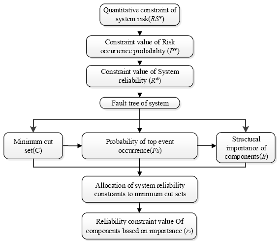
Figure 1.
Flow chart of reliability constraint value allocation based on risk constraints and importance
2.2. Sequential Inspection Model based on Real-Time Reliability
In this paper, the gyroscope of inertial navigation system used in the aviation product is taken as the research object. It is found that the degradation processes of many aviation products’ performance are random and uncertain. The Wiener process can accurately describe the time uncertainty of the degradation process, and it is also easier to deal with the error of data measurement. Due to the long service life and high cost of maintenance of aviation products, periodic inspection or real-time monitoring is generally required. If the performance degradation is found to exceed the failure threshold, the component will be replaced immediately. The diagram of inspection and maintenance cycle is shown in Figure 2.
Figure 2
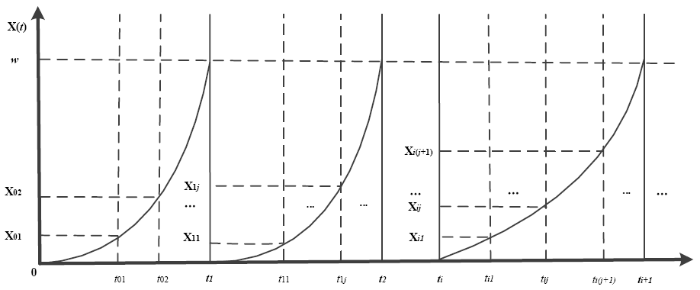
Figure 2.
Inspection and maintenance cycle diagram for the product
The Wiener process is used to establish the degradation model of aviation products. ${{R}_{S}}(t|{{x}_{k}})$ is defined as the real-time reliability at time $t$. According to the definition of real-time reliability, the value of ${{R}_{S}}(t|{{x}_{k}})$ would gradually decrease from 1 after each inspection as time goes on, and the process is thus divided into three steps based on the sequential inspection policy. Firstly, the real-time reliability model is established based on Wiener process; then, the model parameters are estimated by using the degradation data ${{x}_{i(0:k)}}$, so the PDF expression ${{f}_{{{L}_{k}}|{{X}_{0:k}}}}({{l}_{k}}|{{X}_{0:k}})$ of the remaining life for the product can be obtained.Furthermore, the expression ${{R}_{S}}({{l}_{ik}}|{{X}_{0:k}})$ of the real-time reliability can be derived. Finally, the inspection interval $\Delta {{t}_{ik}}$ is determined to satisfy the requirement of reliability constraint value ${{r}^{*}}$ of the component, so the next inspection time is ${{t}_{i(k+1)}}={{t}_{ik}}+\Delta {{t}_{ik}}$.
3. Methodology
3.1. Establishment of the System Fault Tree
Taking the inertial navigation system as an example, there are two reasons for the failure of the inertial navigation system T, which are the factors A and B. The fault tree of the inertial system is established by analyzing the structure and function of the inertial platform, and it is shown in Figure 3.
Figure 3
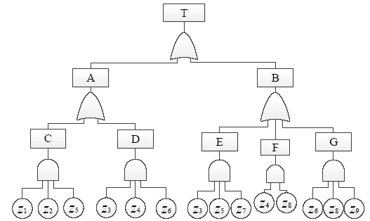
Figure 3.
Fault tree model of inertial navigation system
The Fussell-Vesely method is used to find all the minimum cut sets of the fault tree, and five minimum cut sets of the fault tree can be obtained: {C, D, E, F, G}. According to the non-Boolean algebraic method, the probability function FS of the top event can be obtained:
Here, ${{F}_{i}},\text{ }(i=1,2,\cdots ,9)$ is the unreliability of each basic component. When the reliability of each component in the system is unknown, the structural importance can be used to analyze the fault tree. The structural importance only considers the position of each bottom event in the fault tree, and there is no relationship with its reliability. Assuming that the initial unreliability of all components in the fault tree is ${{F}_{i}}=0.5,\text{ }(i=1,2,\cdots ,9)$, then the structural importance is equal to the probability importance, that is:
3.2. Determination of the Component Reliability Constraint Value
The initial value of the reliability of each component that makes up the minimum cut set is setas ${{r}_{i0}}$, and then the reliability of each minimum cut set can be obtained as follows:
The system reliability ${{R}_{S}}$ can be expressed as follows:
According to literature [15] and the principle of reliability allocation, the low reliability ${{R}_{1}},{{R}_{2}},\cdots ,{{R}_{{{k}_{0}}}}$ should be raised to a certainvalue ${{R}_{0}}$, while the original ${{R}_{{{k}_{0}}+1}},\cdots ,{{R}_{n}}$ with higher reliability remain unchanged. Furthermore, ${{R}_{S}}$ should meet the requirement of constraint value ${{R}^{*}}$ of system risk, namely:
Where ${{k}_{0}}$ represents the number of minimum cut set needed to improve the reliability, ${{k}_{0}}$ is determined by trial and error method, and ${{R}_{0}}$ needs to satisfy the inequality ${{R}_{{{k}_{0}}}}<{{R}_{0}}<{{R}_{{{k}_{0}}+1}}$; thus, the reliability requirement of each minimum cut set can be determined. Then, the reliability requirements will be assigned to each basic event according to the structural importance. $I_{i}^{St}$ is defined as the importance of each basic event, the initial reliability of each basic event is set as ${{r}_{i0}}=0.5,\text{ (}i=1,2,\cdots ,9)$, and $\Delta {{r}_{i}},\text{ }(i=1,2,\cdots ,m)$ represents the reliability of each basic event that needs to be improved; therefore, the reliability that should be assigned to the basic components is ${{r}_{i}}={{r}_{i0}}+\Delta {{r}_{i}}$. For the basic events of high importance, the increment of the assigned reliability should also be larger. Therefore, it is reasonable that the increment and the importance of each event depend on the following proportion:
According to Equations (4), (5), and (8), the following conditions are given for the quantitative constraints of system risk based on the actual project:
By solving the equations, we can get the values of $\Delta {{r}_{1}},\Delta {{r}_{2}},\cdots ,\Delta {{r}_{m}}$, then the value of ${{r}_{i}}={{r}_{i0}}+\Delta {{r}_{i}},\text{ }(i=1,2\cdots ,9)$ is further obtained, and ${{r}_{i}}$ is the reliability constraint value of each component, denoted as $r_{i}^{*}$. When multiple minimum cut sets contain the same basic component, multiple reliability constraint values of the component will be obtained, and the maximum value of these should be the final reliability constraint value of the component.
3.3. Real-Time Reliability Evaluation of the Component
For a running inertial navigation system, its real-time reliability needs to be assessed in order to carry out related inspection and maintenance activities. In this paper, the gyroscope is taken as the research object. If it is known that the gyroscope has not failed at the current moment, a conditional probability can be used to indicate the reliability level of the gyroscope. When the new degenerated data is obtained, the real-time reliability is further updated. The Wiener process is used to describe the degradation process of the gyroscope's drift data. Based on the theory of the first-hitting time [16], the product is considered invalid when the drift data $\{X(t),\text{ }t\ge 0\}$ first reaches the failure threshold $w,$ so we can use Equation (10) to measure the real-time reliability of the gyroscope:
Where ${{\theta }_{k}}={{\left( {{a}_{k}},{{D}_{k}},{{Q}_{k}},{{\sigma }_{k}}^{2} \right)}^{T}}$.In order to get the expression of $R(t;{{X}_{0:k}},{{\theta }_{k}})$, the definition of the remaining life for the product is given firstly:
Therefore, $R(t,{{X}_{0:k}},{{\theta }_{k}})$ can be expressed as follows:
Based on the adaptive algorithm in [18], combining the strong tracking filtering algorithm, the RTS smoothing algorithm, and the EM algorithm, the parameter estimation ${{\hat{\theta }}_{k}}={{(a_{0k}^{(i+1)},D_{0k}^{(i+1)},Q_{k}^{(i+1)},({{\sigma }^{2}})_{k}^{(i+1)})}^{T}}$ based on the degradation inspection data ${{X}_{0:k}}$ can be adaptively updated.
3.4. Determination of Sequential Inspection Intervals
It can be seen that when the relevant parameters are obtained, the predicted value of product performance degradation and the real-time reliability of the remaining life can be obtained at each measurement point. Specifically, in order to make the model parameters converge faster and achieve higher accuracy in the case of small sub-samples, the approximate initialization parameters ${{\theta }_{0}}={{({{a}_{0}},{{D}_{0}},{{Q}_{0}},\sigma _{0}^{2})}^{T}}$ required in the EM algorithm can be calculated according to the historical data of similar products. For a gyroscope, which is an important part of the inertial navigation system, the requirement of real-time reliability is determined as ${{r}^{*}}$ (constant) according to the proposed method in Section 2, and the degradation threshold of drift coefficient is represented by $w$. The specific analysis process of sequential inspection and maintenance based on the real-time reliability requirements ${{r}^{*}}$ is shown as follows:
3.4.1. Determination of the Initial Inspection Time t01 and t02for the New Gyroscope
In order to estimate the parameter ${{\hat{\theta }}_{k}}$ more accurately and make parameter estimation converge more quickly, two state information of the product are required at least. Conservatively, the interval for the first inspection is set to be the same as the second inspection considering the product safety and reliability, i.e., ${{t}_{01}}\text{=}{{t}_{02}}/2$. The real-time reliability should be guaranteed before the next inspection, so the following expression is based on Equation (13):
Thus, the second inspection time ${{t}_{02}}$ satisfies the following formula:
Based on the monotonicity of the distribution function, it is easy to get the solution $\bar{t}_{02}$ of the unary equation by using MATLAB, then ${{t}_{02}}\le {{\hat{t}}_{02}}$. According to engineering practice, the second inspection time can be set as ${{t}_{02}}={{\hat{t}}_{02}}$, so the first inspection time is ${{t}_{01}}={{t}_{02}}/2={{\hat{t}}_{02}}/2$, and then the product can be respectively inspected at ${{t}_{01}}$ and ${{t}_{02}}$ to obtain new degradation data ${{x}_{01}}$ and ${{x}_{02}}$.
3.4.2. Determination of the Inspection Time ${{t}_{i(k+1)}},\text{ }(i\ge 0,\text{ }k\ge 0)$
After obtaining the product degradation data ${{x}_{01}}$ and${{x}_{02}}$, the new parameter ${{\hat{\theta }}_{\text{01}}}$ can be determined by using the adaptive estimation method to integrate ${{x}_{01}}$ and ${{\theta }_{0}}$. Similarly, the parameter ${{\hat{\theta }}_{\text{02}}}$ is adaptively estimated by integrating the degradation data ${{x}_{01}}$, ${{x}_{02}}$ and parameter ${{\hat{\theta }}_{\text{01}}}$, and then the inspection interval $\Delta {{\hat{t}}_{02}}$ can be determined according to the requirement of ${{r}^{*}}$, so the third inspection time is ${{t}_{03}}={{t}_{02}}+\Delta {{\hat{t}}_{02}}$.
If the degradation data of the next inspection still does not exceed the failure threshold $w$, the new inspection data ${{x}_{0k}}$ and parameter ${{\hat{\theta }}_{0(k-1)}}$ will be integrated to estimate the parameter ${{\hat{\theta }}_{0k}}$ recursively, and then the interval after each inspection can be determined. Similarly, the next inspection time will meet the following condition:
For further consideration, if the degradation data ${{x}_{0n}}$ exceeds the failure threshold $w$ during the inspection, this component will be replaced. Then, all the degradation data ${{x}_{(i-1)(0:n)}}$ of inspections after the $(i-1)$th, $(i\ge 1)$ maintenance is used to estimate the parameter ${{\hat{\theta }}_{i0}}$ adaptively, and ${{\hat{\theta }}_{i0}}$ will be taken as the initial parameter of the model after the ith maintenance. Similarly, all the inspection data ${{x}_{i(0:k)}}$ is used to estimate the model parameters ${{\hat{\theta }}_{ik}}$ adaptively, so then the interval $\Delta {{t}_{ik}}$ can be determined, and the interval $\Delta {{t}_{ik}}$ satisfies the following condition:
Similarly, $\Delta {{\hat{t}}_{ik}}$ can be easily obtained by using MATLAB, so there is:
4. Numerical Example
4.1. Determination of Gyroscope Reliability Constraint Value
Assuming the failure of an inertial navigation system will result in an economic loss of 1,000,000 USD for aviation equipment, the risk loss of engineering requirement should be controlled within 100,000 USD during inspection and maintenance. Therefore, the failure probability is P*=0.1, and the system reliability threshold is ${{R}^{*}}=0.9$. When the initial reliability of all basic components is 0.5, the reliability of the five minimum cut sets should be increasedto ${{R}_{0}}={{0.9}^{(1/5)}}=0.9791$. In addition, when the initial reliability of all basic components is 0.5, the structure importance of each component is equal to the probability importance, and then
$I_{1}^{St}=0.191,\text{ }I_{2}^{St}=0.191,\text{ }I_{3}^{St}=0.035$
$I_{4}^{St}=0.0195,\text{ }I_{5}^{St}=0.223,\text{ }I_{6}^{St}=0.0117$
$I_{7}^{St}=0.0039,\text{ }I_{8}^{St}=0.0117,\text{ }I_{9}^{St}=0.0039$
Substituting ${{R}_{0}}=0.9791$ into Equation (9) in Section 3.2, the reliability constraint value of each component is:
${{r}_{1}}=0.713,\text{ }{{r}_{2}}=0.713,\text{ }{{r}_{3}}=0.831$
${{r}_{4}}=0.917,\text{ }{{r}_{5}}=0.903,\text{ }{{r}_{6}}=0.774$
${{r}_{7}}=0.507,\text{ }{{r}_{8}}=0.774,\text{ }{{r}_{9}}=0.591$
In the inertial navigation system, the component Z5 is the gyroscope, so then the real-time reliability threshold of gyroscopeis r*=r5=0.903, which will be used in the analysis process of sequential inspection and maintenance.
4.2. Evaluation of Gyroscope Real-Time Reliability Model
Gyroscopes in inertial navigation systems are very expensive and can only be subjected to limited experiments to obtain degradation data. Since gyroscope drift has an effect on the accuracy of inertial navigation systems, once the drift data exceeds the failure threshold $w$, a new gyroscope must be replaced to ensure the INS’s accuracy. The failure threshold of gyroscope drift is setas $w=0.6({}^\circ /h)$. Firstly, the approximate initial parameter ${{\hat{\theta }}_{0}}={{(0.04426,0.00017,0.00737,0.00053)}^{T}}$ is obtained by integrating the drift data of the same type product. In order to verify the effectiveness of the model proposed in this paper, we select the drift data information corresponding to time ${{t}_{1:90}}$ as the degradation data. For each inspection time, the degradation information ${{X}_{1:h}}$ before the inspection time is set as the history degradation information; thus, the parameter of the degradation model can be updated by using the adaptive estimation method, and then the future drift data of the gyroscope can be predicted by the formula ${{\hat{x}}_{k+1}}={{x}_{k}}+{{\hat{\mu }}_{k}}({{t}_{k+1}}-{{t}_{k}})$ step by step. Finally, the result is compared with the real curve of drift data growth for the gyroscope. The comparison is shown in Figure 4.
Figure 4
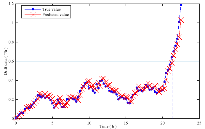
Figure 4.
The comparison plot of drift data curve
According to the result of the experiment, the theoretical failure time of the gyroscope is about 21.5h, and the mean square error between the predicted value and the true value is $MSE=1.852\times {{10}^{-4}}$. It can be seen that the model proposed in this paper fits very well with the real model.
4.3. Sequential Inspection Intervals
The calculation process of the sequential inspection interval is given as follows: Firstly, ${{r}^{*}}$ is set as ${{r}^{*}}=0.903$. ${{t}_{02}}\text{=9}\text{.4224}$ can be obtained by using the method proposed in Section 3.4, so ${{t}_{01}}={{t}_{02}}/2=4.7112$. Secondly, when $i=0,k=1,2$, ${{\hat{\theta }}_{01}}={{({{a}_{01}},{{D}_{01}},{{Q}_{01}},\sigma _{01}^{2})}^{T}}$ and ${{\hat{\theta }}_{02}}={{({{a}_{02}},{{D}_{02}},{{Q}_{02}},\sigma _{02}^{2})}^{T}}$ are respectively estimated by the adaptive estimation method. Thirdly, the inspection interval $\Delta {{\hat{t}}_{ik}}$ is determined according to the requirement of real-time reliability ${{r}^{*}}$, i.e., ${{t}_{i(k+1)}}={{t}_{ik}}+\Delta {{\hat{t}}_{ik}}$; when $i=0,\text{ }k=2$, ${{t}_{03}}$ is obtained; when $i=0,\text{ }k=3$, ${{t}_{04}}$ is obtained. If the drift data exceeds the failure threshold, the product will be replaced immediately. In the second operating phase, the parameter ${{\hat{\theta }}_{05}}$ of the first phase is taken as the initial parameter and the parameters are recursively updated. Then, the time of each inspection and maintenance can be determined, and the following inspection time will be obtained in the same way. The inspection time ${{t}_{ik}}$ determined by the proposed sequential method is shown in the second row of Table 1, and the third row shows the degradation data ${{x}_{ik}}$ of each inspection. Finally, the following results can be obtained from the numerical example:
Table 1. The calculation results of sequential inspection interval (${{r}^{*}}=0.903$)
| The serial number | ${{t}_{ik}}/h$ | ${{x}_{ik}}/({}^\circ /h)$ | ${{a}_{ik}}$ | ${{D}_{ik}}$ | ${{Q}_{ik}}$ | ${{({{\sigma }^{2}})}_{ik}}$ | $\Delta {{\hat{t}}_{ik}}/h$ | Remarks |
|---|---|---|---|---|---|---|---|---|
| The initial state (${{t}_{0}}=0$) | 0.00000 | 0.00000 | 0.04426 | 0.00017 | 0.00737 | 0.00053 | 4.71120 | The degradation data exceeds the failure threshold 0.6 $({}^\circ /h)$ at the sixth inspection, which needs to be replaced. |
| ${{t}_{01}}$ | 4.7112 | 0.19203 | 0.04419 | 0.00016 | 0.00028 | 0.00083 | 4.71120 | |
| ${{t}_{02}}$ | 9.4224 | 0.35605 | 0.04273 | 0.00012 | 0.00015 | 0.00059 | 3.80590 | |
| ${{t}_{03}}$ | 13.2283 | 0.27352 | 0.04106 | 0.00008 | 0.00100 | 0.00434 | 3.38730 | |
| ${{t}_{04}}$ | 16.6156 | 0.31776 | 0.04068 | 0.00007 | 0.00068 | 0.00356 | 3.01020 | |
| ${{t}_{05}}$ | 19.6258 | 0.30006 | 0.04012 | 0.00007 | 0.00050 | 0.00285 | 3.58900 | |
| ${{t}_{06}}$ | 23.2148 | 1.84797 | —— | —— | —— | —— | —— | |
| Replace as new (${{t}_{1}}$) | 23.2148 | 0.00000 | 0.04012 | 0.00007 | 0.00050 | 0.00285 | 8.75680 | The degradation data exceeds the failure threshold at the fifth inspection, which needs to be replaced. |
| ${{t}_{11}}$ | 31.9716 | 0.28173 | 0.03950 | 0.00006 | 0.00024 | 0.00104 | 5.26090 | |
| ${{t}_{12}}$ | 37.2325 | 0.19451 | 0.03773 | 0.00005 | 0.00101 | 0.00657 | 4.05290 | |
| ${{t}_{13}}$ | 41.2854 | 0.31754 | 0.03721 | 0.00005 | 0.00068 | 0.00546 | 2.60630 | |
| ${{t}_{14}}$ | 43.8917 | 0.49501 | 0.03660 | 0.00005 | 0.00052 | 0.00515 | 0.54880 | |
| ${{t}_{15}}$ | 44.4405 | 0.62656 | —— | —— | —— | —— | —— | |
| Replace as new (${{t}_{2}}$) | 44.4405 | 0.00000 | 0.03660 | 0.00005 | 0.00052 | 0.00515 | 7.92460 | The degradation data exceeds the failure threshold at the fourth inspection, which needs to be replaced. |
| ${{t}_{21}}$ | 52.3651 | 0.20505 | 0.03616 | 0.00005 | 0.00032 | 0.00122 | 6.86210 | |
| ${{t}_{22}}$ | 59.2272 | 0.20363 | 0.03453 | 0.00004 | 0.00031 | 0.00273 | 5.85850 | |
| ${{t}_{23}}$ | 65.0857 | 0.49155 | 0.03359 | 0.00004 | 0.00025 | 0.00410 | 0.69760 | |
| ${{t}_{24}}$ | 65.7833 | 0.66387 | —— | —— | —— | —— | ||
| … | … | ... | … | … | … | ... |
If the gyroscope is not inspected, the theoretical service life will be about 8.7 hours when r*=0.903. However, if the sequential inspection method is used, the effective service life of the material is about 21 hours, which is close to the theoretical failure time of 21.5 hours. The service life of aviation products is extended effectively.
As shown in Table 1, the sequential inspection interval is not equal spacing, and the number of inspections is reduced from 6 times to 5 times after one maintenance and to 4 times after two maintenances. As the data accumulates, the number of inspections can be further reduced. Therefore, the sequential inspection method proposed in this paper can not only effectively reduce the number of inspections, but also improve the efficiency of inspection and maintenance while ensuring the reliability of aviation products.
It can be seen that the convergence rate of model parameters is very fast in the case of small sample data, and the prediction accuracy also meets requirements of real applications.
5. Conclusions
In this paper, a sequential inspection model based on risk quantitative constraint and component importance for aviation products has been proposed. System reliability is determined based on the quantitative constraint of system risk, and then according to the structure importance of each component,the system reliability is assigned to each basic component. Thus, the system risk quantitative constraint is converted into the reliability constraint of the basic component. Developing related sequential inspection and maintenance strategies based on the component reliability constraint not only makes the system inspection and maintenance becomesimple and feasible, but also controls the overall risk of system within the scope of the actual engineering requirement.In addition, it is known that in the actual operation process of aviation products, the mechanism of performance degradation is complex and the degradation process shows randomness. The sequential inspection method can adaptively update the relevant parameters of the degradation model in real time so that the time of each inspection and maintenance can be determined more accurately. The method can not only ensure the reliability of the product, but also avoid the problems of over-inspection and under-inspection that may be caused by the traditional equal-pitch cycle inspection. The number of inspection data is also required less by the sequential inspection method. Moreover, the convergence rate of relevant parameters becomes faster by integrating the historical information of the same type products, and the model has good robustness so as to ensure the reliability requirement and the prediction accuracy of the aviation products, which is very suitable for the determination of inspection and maintenance intervals of the new small-sample product.
The research of this paper is carried out under the condition of considering the perfect maintenance for the product. In some cases, the performance of the product as a whole is affected by other non-replaceable parts and some environmental factors, so the performance cannot recover as new after maintenance. Therefore, further studies will consider the inspection method for the products in the case of imperfect maintenance.
Acknowledgements
This research is supported by the project of the Natural Science Foundation of China (No. 61573370).
Reference
Risk-based Optimization of Pipe Inspections in Large Underground Networks with Imprecise Information
,”
Development of a Risk-based Maintenance Strategy Using FMEA for a Continuous Catalytic Reforming Plant
,”
DOI:10.1016/j.jlp.2012.05.009
URL
[Cited within: 1]

Petrochemical facilities and plants require essential ongoing maintenance to ensure high levels of reliability and safety. A risk-based maintenance (RBM) strategy is a useful tool to design a cost-effective maintenance schedule; its objective is to reduce overall risk in the operating facility. In risk assessment of a failure scenario, consequences often have three key features: personnel safety effect, environmental threat and economic loss. In this paper, to quantify the severity of personnel injury and environmental pollution, a failure modes and effects analysis (FMEA) method is developed using subjective information derived from domain experts. On the basis of failure probability and consequence analysis, the risk is calculated and compared against the known acceptable risk criteria. To facilitate the comparison, a risk index is introduced, and weight factors are determined by an analytic hierarchy process. Finally, the appropriate maintenance tasks are scheduled under the risk constraints. A case study of a continuous catalytic reforming plant is used to illustrate the proposed approach. The results indicate that FMEA is helpful to identify critical facilities; the RBM strategy can increase the reliability of high-risk facilities, and corrective maintenance is the preferred approach for low-risk facilities to reduce maintenance expenditure.
An Evaluation of Maintenance Strategy Using Risk based Inspection
,”
DOI:10.1016/j.ssci.2011.01.015
URL
[Cited within: 1]
Risk based inspection (RBI) methodology was proposed to evaluate the maintenance strategy in industrial process which was constructed in one of the units of Fujian Oil Refinery ISOMAX unit. Using classic definition of risk, both the probability and consequence of accident or failure were investigated respectively under the support of risk-specific code. All equipment in this unit were evaluated and categorized into five risk zone based on the RBI result which covered five levels. In addition, an application of the analytical hierarchy process (AHP) to select the most practicable maintenance strategy for equipment which was located in each risk rating scale was described. To arrange the hierarchic structure and evaluation, four main criteria were defined for pairwise judgments. Finally, four possible alternative strategies were proposed for administrators on the site.
Development of a Risk-based Maintenance (RBM) Strategy for a Power-Generating Plant
,”
DOI:10.1016/j.jlp.2005.01.002
URL
[Cited within: 1]
The unexpected failures, the down time associated with such failures, the loss of production and, the higher maintenance costs are major problems in any process plant. Risk-based maintenance (RBM) approach helps in designing an alternative strategy to minimize the risk resulting from breakdowns or failures. Adapting a risk-based maintenance strategy is essential in developing cost-effective maintenance policies. The RBM methodology is comprised of four modules: identification of the scope, risk assessment, risk evaluation, and maintenance planning. Using this methodology, one is able to estimate risk caused by the unexpected failure as a function of the probability and the consequence of failure. Critical equipment can be identified based on the level of risk and a pre-selected acceptable level of risk. Maintenance of equipment is prioritized based on the risk, which helps in reducing the overall risk of the plant. The case study of a power-generating unit in the Holyrood thermal power generation plant is used to illustrate the methodology. Results indicate that the methodology is successful in identifying the critical equipment and in reducing the risk of resulting from the failure of the equipment. Risk reduction is achieved through the adoption of a maintenance plan which not only increases the reliability of the equipment but also reduces the cost of maintenance including the cost of failure.
Quantitative Risk Prognostics Framework based on Petri Net and Bow-Tie models
,”
DOI:10.1016/j.ress.2017.03.026
URL
[Cited within: 1]
A simulation framework based on the Petri Net model is proposed in this paper used for performing quantitative risk prognosis through extending the Bow-Tie model. A Petri Net model is built to include features, specific to assets, such as the condition of the asset, the projected operational usage, inspection and maintenance policies and degradation process, so that the future condition of the asset over time can be estimated. Several new Petri Net modelling features which advance the traditional Bow-Tie approach are proposed, such as asset usage generating and usage dependent transitions, and the possibility of entering evidence about the actual condition of the asset through the use of truncated distributions. Monte Carlo simulation method is used to simulate the developed Petri Net model over a selected time frame, in order to obtain statistics necessary to perform risk assessment using the Bow-Tie model. The paper reports on the overall proposed methodology and then focusses on the development of the Petri Net model. The methodology is applied in risk prognostics of operating an underground passenger lift. In particular, the combination of the Petri Net and the Bow-Tie models is illustrated to predict the likelihood and the consequences of an event when a lift gets stuck in a shaft between landings.
A New Class of Wiener Process Models for Degradation Analysis
,”
DOI:10.1016/j.ress.2015.02.005
URL
[Cited within: 1]
61We propose a new Wiener process to capture dependence between mean and variance.61Random-effects Wiener process models are developed so that the variance is increasing in the degradation mean.61Stress are incorporated into the process in a similar way.61Statistical inference methods are also developed.61The methods are applied to two real examples.
A Wiener Process Model for Accelerated Degradation Analysis Considering Measurement Errors
,”
DOI:10.1016/j.microrel.2016.08.004
URL
[Cited within: 1]
61A generalized Wiener process model is proposed for modeling accelerated degradation test.61The explicit form of the probability distribution function (PDF) are derived based on the concept of first hitting time.61Maximum likelihood method with genetic algorithm (GA) is adopted to estimate the unknown parameters.61A comprehensive simulation and a real LED example are given to illustrate the benefits of the proposed model.
Optimal Inspection and Replacement Policies for Multi-Unit Systems Subject to Degradation
,”
DOI:10.1109/TR.2017.2778283
URL
[Cited within: 1]
Condition-based maintenance (CBM) is proved to be effective in reducing the long-run operational cost for a system subject to degradation failure. Most existing research on CBM focuses on single-unit systems where the whole system is treated as a black box. However, a system usually consists of a number of components and each component has its failure behavior. When degradation of the components is observable, CBM can be applied to the component level to improve the maintenance efficiency. This paper aims to study the optimal inspection/replacement CBM strategy for a multi-unit system. Degradation of each component is assumed to follow a Wiener process and periodic inspection is considered. We cast the problem into a Markov decision framework and derive the optimal maintenance decisions that minimize the maintenance cost. To better illustrate the optimal maintenance strategy, we start from a 1-out-of-2: G system and show that the optimal maintenance policy is a two-dimensional control limit policy. The argument used in the 1-out-of-2: G system can be readily extended to general cases in a similar way. The value iteration algorithm is used to find the optimal control limits, and the optimal inspection interval is subsequently determined through a one-dimensional search. A numerical study and a comprehensive sensitivity analysis are provided to illustrate the optimal maintenance strategy.
Real-Time Reliability Evaluation of Two-Phase Wiener Degradation Process
,”
DOI:10.1080/03610926.2014.988262
URL
[Cited within: 1]
Reliability modeling and evaluation for the two-phase Wiener degradation process are studied. For many devices, the degradation rates could possibly increase or decrease in a non smooth manner at some point in time due to the change of degradation mechanism. A two-phase Wiener degradation process with an unobserved change point is used to model the degradation process. And we assume that the change point varies randomly from device to device. Furthermore, we integrate historical data and up-to-date observation data to improve the degradation modeling and evaluation based on Bayesian method. The change point between the two phases was obtained based on the Akaike information criterion (AIC) and the criterion of the residual sum of squares. Finally, a real example of liquid coupling devices (LCDs) and a numeric example are discussed to demonstrate the effectiveness of the proposed method. The results show that the proposed method is effective and efficient.
Real-Time Reliability Assessment based on Acceleration Monitoring for Bridge
,”
DOI:10.1007/s11431-016-6059-5
URL
[Cited within: 1]
Bridge health monitoring (BHM) has become increasingly significant in the life-cycle of the structure such as maintenance, repair and rehabilitation. It is necessary to use BHM information efficiently to assess the working conditions of the bridge. The main objective of this study is to develop an effective method and establish a framework for the real-time reliability assessment based on BHM acceleration information. The first-passage probability and its further development have been proposed to assess the reliability probability. The first-passage probability shows the probability of that a scalar process exceeds a designated threshold during a given time interval. The advantage of the proposed method is the assessment of the real-time reliability probability based on the monitoring information during an assessment reference period. Furthermore, the velocity data and displacement data are calculated from the acceleration monitoring data using the relationships between their power spectral density (PSD) functions. The real-time reliability assessment of Donghai Bridge, which is the first large scale cross-sea bridge in China, demonstrates that the proposed method is efficient and effective.
A Study on the Real-Time Reliability of on-Board Equipment of Train Control System
,”DOI:10.1088/1757-899X/351/1/012004 URL [Cited within: 1]
Sequential Inspection Method for Long-Storage-Products based on Storage Degradation Mechanism
,”In order to specify the optimal inspection way for long-storage-products,such as engine,under storage reliability requirement,the sequential inspection method based on storage degradation mechanism was proposed.The storage degradation mechanism covers the aging of non-repairable components and degradation of repairable components despite of the inspection and maintenance.The storage reliability model for Weibull products and its parameters estimation methods with least square errors were proposed.Sequential inspection time was confirmed based on storage reliability request and virtual storage life.At last,a simulation example was given to illustrate the validity of the method.
Approximate Methods for Optimal Replacement, Maintenance, and Inspection Policies
,”
DOI:10.1016/j.ress.2015.07.005
URL
[Cited within: 1]
61The failure times are obtained approximately in a simpler equation form.61Age and periodic replacement models and their optimal solutions are obtained approximately in an easier way.61Approximate imperfect maintenance times are close to the exact optimal solutions.61The approximate MTTF is used to easily obtain optimal number of units needed for a parallel system.61Approximate computation for the sequential inspection times is proposed.
Optimization of Alarm Threshold and Sequential Inspection Scheme
,”
DOI:10.1016/j.ress.2009.09.012
URL
[Cited within: 1]
An item is subject to gradual degradation. The degradation can be represented by a measurable, non-negative and non-decreasing quantity. The item can be in one of three different states: normal (when the degradation quantity is smaller than a threshold of alarm or potential failure), functional failure (when the degradation quantity is larger than a functional failure threshold) and in-between or potential failure (when the degradation quantity is larger than the alarm threshold and smaller than the functional failure threshold). A sequential inspection scheme is implemented to determine the state of the item so as to prevent a functional failure. The paper presents a flexible degradation model and two cost models to optimize the alarm threshold and the sequential inspection scheme. The usefulness and appropriateness of the proposed models are illustrated by examples.
New Approach on System Reliability Distribution by Component Importance in FTA
,”The reliability distribution of complex system is one of unsolved issues in system safety engineering.In this paper,the Fault Tree Analysis(FTA) is introduced into the system reliability distribution.It would be more reasonable to distribute the reliability from system to basic events(components) according to the value of the component importance.There are two steeps to achieve the reliability distribution.First,the target reliability of a system is distributed to all the minimum cut sets based on reliability distribution theory.The reliability of a minimum cut set is then distributed to the basic events in this cut set if the reliability of this cut needs to be adjusted.This reliability distribution method can be used not only for a simple system where the components are connected in series or in parallels,or both,but also for a complex system,such as the bridge connection presented in this system.
Threshold Regression for Survival Analysis: Modeling Event Times by a Stochastic Process Reaching a Boundary
,”
Mis-specification Analysis of Linear Degradation Models
,”
DOI:10.1109/TR.2009.2026784
URL
[Cited within: 1]
Degradation models are widely used to assess the lifetime information of highly reliable products if there exists quality characteristics whose degradation over time can be related to reliability. The performance of a degradation model depends strongly on the appropriateness of the model describing a product's degradation path. In this paper, motivated by laser data, we propose a general linear degradation path in which the unit-to-unit variation of all test units can be considered simultaneously with the time-dependent structure in degradation paths. Based on the proposed degradation model, we first derive an implicit expression of a product's lifetime distribution, and its corresponding mean-time-to-failure (MTTF). By using the profile likelihood approach, maximum likelihood estimation of parameters, a product's MTTF, and their confidence intervals can be obtained easily. In addition, laser degradation data are used to illustrate the proposed procedure. Furthermore, we also address the effects of model mis-specification on the prediction of the product's MTTF. It shows that the effect of the model mis-specification on the predictions of a product's MTTF is not critical under the case of large samples. However, when the sample size and the termination time are not large enough, a simulation study shows that these effects are not negligible.
