


1. Introduction
Residual life prediction of long-term storage products is an important problem currently, especially considering regular testing and preventive maintenance, and it is significant for product health management and equipment production. During the storage time, which consists of the storage period and the inspection period, performance degradation exists in some of the products. The storage period is long, and degradation increases slowly. The inspection period is short, and degradation increases obviously.
For the residual life prediction of specific service equipment, Gao [1] assumed that there is a linear dependence between the exponent ratio and the loading ratio to predict fatigue residual life of materials based on the nonlinear fatigue damage accumulation model. For electromagnetic relays, Zhao [2] proposed a particle filtering-based method for predicting their remaining storage life, which was proven to be effective. Zhang [3] proposed a new residual life prediction method for complex systems based on the Wiener process and evidential reasoning. However, the method is difficult. Based on a similarity-based approach, Blaise [4] used degradation observations depending on acquisition time and reference dataset information built on the knowledge of endurance degradation data to perform prediction. Son [5] conducted a comparative analysis of various residual life prediction methods based on the random coefficient regression model. It is difficult for these methods to reflect the concept of first-time, and this may affect the forecast results.
Regarding maintenance in the degradation process of products, many studies have been carried out. Du [6] proved that timely external maintenance and a sufficient supply of electrolytes can greatly extend the lifespan of storage batteries. Cherkaoui et al. [7] dealt with a quantitative approach to jointly assess the economic performance and robustness of some representatives of time-based and condition-based maintenance. In the maintenance model of Komijani [8], an investigation on the concurrent effects of random shocks during the useful life of the equipment was also studied. Zhang [9] considered the effect of maintenance on the parameters of the degradation process, analysed the residual life of the product under imperfect maintenance, and made maintenance decisions. Yang [10] considered a class of systems with two failure modes, both of which were taken into consideration in the impact of different states of the system. Nourelfath [11] allowed for a joint selection of the optimal values of production plan and the maintenance policy, while taking into account quality-related costs. The research of Lee [12] was based on the assumption that the failure process between two preventive maintenances follows a generalized version of the nonhomogeneous Poisson process. The limitation of these studies is that almost all of them only consider maintenance in a single process.
Considering the multi-stage process, Park [13] believed that it is essential for the multi-stage process monitoring to be able to give a signal at each single stage in order to avoid the delay in detecting assignable causes in the process. Zheng [14] established a staged degradation process model that can describe the effects of incomplete maintenance. Sheng [15] proposed an autoregressive moving average model-filtered hidden Markov model to fit the multi-phase degradation data with an unknown number of jump points. In the current research, most of the studies were conducted to optimize the repair strategy at the same time as the assessment. However, we concentrate on a multi-stage degradation process based on the fixed maintenance strategy.
Overall, in this paper, we analyse the multi-stage degradation process model of long storage products that are regularly tested and repaired, taking full account of the impact of different environmental stresses on the degradation rate of a single product. The simulation method is used to solve the model and determine the residual storage life of products with different degradation parameters. Focusing on the degradation model in multi-stage storage process, we propose a method to predict the residual life of long storage products when considering the amount of degradation of the products to follow the Wiener process. Therefore, this paper provides a way of thinking for the residual life study of long-term storage products considering regular inspection and preventive maintenance.
The rest of the paper is structured as follows. In section 2, a symbol description is presented. Then, we establish the storage model of a single product considering regular inspection and maintenance in section 3. In section 4, we study the prediction of residual life to storage of a single product with regular inspection and preventive maintenance. In section 5, a simulation method is applied to solve the residual life. Finally, the conclusions are given in section 6.
2. Nomenclature
| the diffusion coefficient of the Wiener process | |
|---|---|
| the state of the component | |
| the rate of degradation of the part | |
| the stochastic process of degeneracy | |
| the standard Brownian motion | |
| the storage time at the moment | |
| the length of storage period | |
| the length of inspection period | |
| the time for maintenance | |
| the number of repairs from the beginning of storage to product being failed | |
| the number of repairs at time | |
| the maximum number of preventive maintenance | |
| the failure threshold | |
| the maintenance threshold | |
| the degradation rate during storage period | |
| the degradation rate during detection period | |
| the maintenance effect | |
| the diffusion coefficient of the Wiener process in maintenance period | |
| the point estimation of residual storage life |
3. Model of Degradation Process Considering Maintenance
3.1. Problem Description
In the long-term storage of large-scale equipment systems, performance degradation during storage exists in some of the products, resulting in a direct impact on the availability of products.
The multi-state degradation process includes the storage period and the inspection period. The storage period is a long state when degradation increases slowly. The inspection period is a short state when degradation increases obviously.
At the same time, the structure of this kind of equipment is relatively simple in design and easy to disassemble and install. Therefore, maintaining high availability of products during storage may require several repairs or replacements. The multi-state storage process of product is shown in Figure 1.
Figure 1
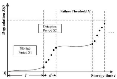
Figure 1.
Degradation process in multi-state storage period
To sample the problem, we make some basic assumptions as follows:
$\cdot$ The maintenance operation takes up negligible time during the entire storage process. In this paper, the main body of the storage process is a natural storage stage, and the process of inspection in it has been relatively short. As an operation in the inspection process, maintenance can be regarded as being completed immediately.
$\cdot$ Maintenance does not affect the parameters of the degradation process. The effect of maintenance on the degradation process is only reflected in the performance degradation values.
$\cdot$ Maintenance can occur at any one moment in the inspection process. Products after the repair do not change the storage state, and their storage state at any time is only related to the pre-determined storage strategy.
3.2. Degradation Model
Due to the good nature of the Wiener process, we use a single-unit linear Wiener process with drift to model the multi-state storage process. Referring to the model description of Si et al. [16],
Where
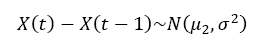
We assume that the inspection start time and the duration in this problem are both fixed values. The natural storage state and the inspection state can be regarded as linear Wiener processes. Therefore, the degradation process can be expressed as the following form:
Where
Therefore, on the condition of knowing the current performance inspection data, the distribution function of the lifetime of products can be expressed as the following conditional distribution function:
From Formula (3) and Formula (4), the residual life of products when stored to time
Similarly, the residual life distribution function of products is
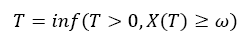
Under the parameter callback method, with
Where
In actual processing, the parameters in the callback amount distribution need to be determined according to the historical maintenance data and the maintenance data of the same type of product. The presentation of the maintenance method is shown in Figure 2.
Figure 2
Figure 2.
Maintenance in storage period
3.3. Estimation of Parameters
Under the parameter callback method, the maintenance parameters that need to be estimated are
Then, the Bayesian estimation method is used to estimate the distribution parameters of the maintenance effect with the use of current maintenance effect data.
Since the distribution of
Assume that the maintenance effect parameters
Therefore, we can get the probability density function of
Next, the prior distribution should be determined. Under the condition of no information, when the distribution of samples is normally distributed, the prior distributions of mean and variance are non-information distribution. Assume that the prior distributions of
$\mu_{m} \sim U(\mu_{m1},\mu_{m2})$ $\sigma^{2}_{m} \sim U(\sigma^{2}_{m1},\sigma^{2}_{m2})$
Due to the assumption of independence, the joint prior density function of
With the prior distribution and likelihood function being obtained, the Bayesian principle can be used to obtain the joint posterior distribution density function of the parameters
Where
If it is necessary to estimate a specific parameter, the joint posterior distribution density function of the parameter
4. Residual Storage Life Prediction
4.1. Prediction Model
In view of the existence of a preventive maintenance ceiling, the distribution of the residual storage life needs to be discussed based on the number of repairs. For a single product, assuming that the maximum number of preventive maintenance is
Where
When the product is stored at time
Where
Hence, the single residual storage life distribution can be expressed as
To solve Formula (17), the number of repairs to product failure after
In a natural storage process, degradation exceeding the failure threshold will not be repaired due to no inspection during the natural storage period. At the beginning of the next inspection period, the degradation is more than the failure threshold. In this case, the product is failed and there no maintenance occurs. Therefore, specific analysis is needed when
First, we solve the probability
Where
Next, we solve the probability
When no maintenance is carried out, the degradation amount does not exceed the maintenance threshold in any inspection period before time
The probability is
$P((X(t)-X(t-1)) <0)=\int_{-\infty}^{0} \frac{1}{\sqrt{2\pi \sigma}} exp(-\frac{(x-\mu)^2}{2\sigma^2})dx$
This denotes that the difference between two neighbouring moments under the values of
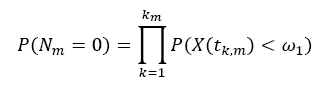
Where
$t_{k,m}=kT=kd, k=1,2,\cdots,k_{m},k_{m}=\frac{t}{T+d}$
which is the most recent test period before time
When
4.2. Prediction Steps
The calculation steps of the prediction method in this paper are as follows:
Step 1 Modeling storage and inspection period.
Define the long-term storage and regular inspection of products, and take into account the determination of degradation parameters
Step 2 Modeling maintenance period.
Define the conditions and completion effects of the maintenance, and take into account the determination of maintenance parameters
Step 3 Performing prediction.
Define the entire degradation process of the product, and take into account the determination of the upper limit of the number of maintenances
The schematic diagram of the prediction process is shown in Figure 3.
Figure 3
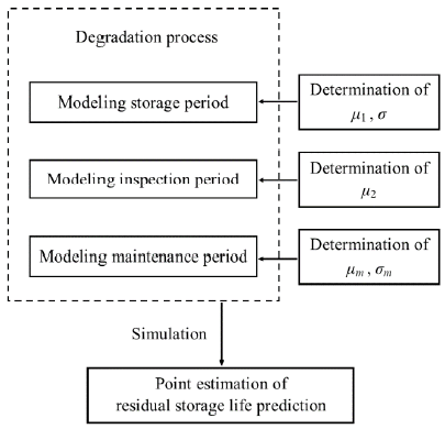
Figure 3.
The prediction process
5. Calculation Examples
In the simulation method, we simulate the storage process according to the probability distribution formulas we have obtained and sampled the statistics to get the distribution of the residual storage life under the simulation scenario. Then, all samples are averaged to get the point estimation of the residual storage life of the product.
5.1. Calculation of Degradation Model
In this part, we set 1000 samples in an experiment when storage time
From Figure 4, it can be seen that the degradation showed the characteristics of fluctuant rise in general. In the storage period, it changes very little. It significantly increases during the inspection period, which is due to the changes of environmental stress during this period. From time 2030 to 2040, when the degradation exceeds the maintenance threshold
Figure 4
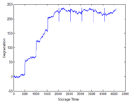
Figure 4.
Example of degradation process in experiment 1
In each experiment, residual life values of all samples are collected. The distributing condition in experiment 1 is shown in Figure 5.
Figure 5
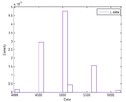
Figure 5.
Residual life distribution in experiment 1
From Figure 5, we can find that the samples concentrate on several values. This is because the degradation in the inspection period is much more significant than that in the storage period, and maintenance times are limited. Therefore, many products fail upon reaching the upper limit of repair times, causing the relatively concentrated sample values of storage life.
5.2. Comparison Experiments
To compare the effect of different degradation parameters, residual storage life estimation
In experiment 2, we change
In experiment 3, we change
In experiment 4, we change
In experiment 5, we change
The cumulative distribution functions of all experiments are shown in Figure 6.
Figure 6
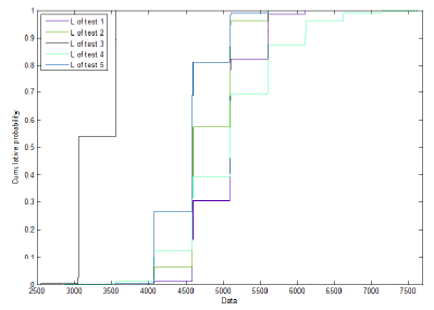
Figure 6.
The cumulative distribution functions of residual storage life
As shown in Figure 6, in each experiment, the cumulative probability curve seems to be stepped, the reason of which is the same as that of the samples concentrating on several values in Figure 5. In addition, the leftmost curve in them belongs to test 3. The maximum value of residual storage life occurs in test 4 and reaches 7500 hours approximately.
The prediction results and corresponding parameter settings of all experiments are shown in Table 1.
Table 1. Estimation results for residual storage life
| Experiment number | Degradation parameters | Maintenance parameters | |||||
|---|---|---|---|---|---|---|---|
| 1 | 0.005 | 5 | 0.5 | 50 | 1 | 5019 | |
| 2 | 0.01 | 5 | 0.5 | 50 | 1 | 4796 | |
| 3 | 0.005 | 8 | 0.5 | 50 | 1 | 3291 | |
| 4 | 0.005 | 5 | 1 | 50 | 1 | 5016 | |
| 5 | 0.005 | 5 | 0.5 | 40 | 1 | 4564 | |
From Table 1, besides the prediction values of residual life, we can find the relationship between parameters and residual life. Comparing experiment 1 and experiment 2, residual life is cut down when
6. Conclusions
In this paper, we analyse the multi-stage degradation process model of long storage products that are regularly experimented and repaired, taking full account of the impact of different environmental stresses on the degradation rate of a product.
With the assumption that maintenance can occur at any one moment in the natural inspection process, we consider the product to be regular repaired in the process of storage, so that the storage model can be established. Then, we perform parameters estimation to analyse the influence of storage parameters
Although we discuss preventive maintenance, we focus on multi-stage degradation when considering the amount of degradation of the product to follow the Wiener process. Therefore, this paper provides a way of thinking for the residual life study of long-term storage products considering regular inspection and preventive maintenance to a certain extent.
Acknowledgements
This research is supported by the project of Natural Science Foundation of China (No. 61573370 and 71371182).
Reference
Residual Life Prediction based on Nonlinear Fatigue Damage Accumulation Model
,”
DOI:10.1007/s12204-015-1647-2
URL
[Cited within: 1]

When a nonlinear fatigue damage accumulation model based on damage curve approach is used to get better residual life prediction results, it is necessary to solve the problem caused by the uncertain exponent of the model. Considering the effects of load interaction, the assumption that there is a linear dependence between the exponent ratio and the loading ratio is established to predict fatigue residual life of materials. Three experimental data sets are used to validate the rightness of the proposition. The comparisons of experimental data and predictions show that the predictions based on the proposed proposition are in good accordance with the experimental results as long as the parameters that represent the linear correlativity are set an appropriate value. Meanwhile, the accuracy of the proposition is approximated to that of an existing model. Therefore, the proposition proposed in this paper is reasonable for residual life prediction.
Remaining Storage Life Prediction for an Electromagnetic Relay by a Particle Filtering-based Method
,”
DOI:10.1016/j.microrel.2017.03.026
URL
[Cited within: 1]

In this paper, we propose a particle filtering-based method for predicting the remaining storage life (RSL) of electromagnetic relays. The RSL prediction problem here addressed has the following three distinctive features: i) limited measurement data available; ii) incomplete run-to-failure data; and iii) no model available for the physical degradation process. Then, to develop the method for RSL prediction, storage testing and degradation mechanism analysis have been carried out to obtain the knowledge and information needed to develop the physical model that supports the RSL prediction procedure. We discuss the three main steps of the proposed prediction method: parameter estimation, model validation and RSL prediction. Data from nine relays are used for estimating the initial parameter values distribution and data from one relay are used for RSL prediction. The RSL prediction results are compared with those obtained by a nonlinear curve-fitting method and a basic particle filtering algorithm. The comparison shows that the proposed method is more effective in predicting the RSL than the other methods.
A New Residual Life Prediction Method for Complex Systems based on Wiener Process and Evidential Reasoning
,”
Similarity-based Residual Useful Life Prediction for Partially Unknown Cycle Varying Degradation
,” in
DOI:10.1109/ICPHM.2015.7245054
URL
[Cited within: 1]
Similarity-based approach is a popular data-driven prognostic method for Residual Useful Life (RUL) Prediction. The principle of this approach is based on the “similarity” between the monitored part, i.e., the sample whose the RUL has to be predicted and degradation reference trajectory patterns (or known library of a priori degradation functions). The challenge addressed in this paper concerns the RUL estimation of a test sample using degradation observations depending on acquisition time and reference dataset information, built on the knowledge of endurance degradation data. The “similarity” coefficient is estimated here using a mapping function between the aperiodic time degradation function and the known test cycle functions. Our approach is evaluated on the very classical Virkler crack-growth measurements benchmark [14] and the experimental results show that it is efficiency and promising in the context of railways maintenance.
Evaluation and Comparison of Mixed Effects Model based Prognosis for Hard Failure
,”
DOI:10.1109/TR.2013.2259205
URL
[Cited within: 1]
Failure prognosis plays an important role in effective condition-based maintenance. In this paper, we evaluate and compare the hard failure prediction accuracy of three types of prognostic methods that are based on mixed effect models: the degradation-signal based prognostic model with deterministic threshold (DSPM), with random threshold (RDSPM), and the joint prognostic model (JPM). In this work, the failure prediction performance is measured by the mean squared prediction error, and the power of prediction. We have analyzed characteristics of the three methods, and provided insights to the comparison results through both analytical study and extensive simulation. In addition, a case study using real data has been conducted to illustrate the comparison results as well.
Maintenance of Storage Batteries in Automatic Meteorological Observation Stations
,”Firstly,the definition,structure and working principles of storage batteries in automatic meteorological observation stations were stated simply,and then the daily maintenance of the storage batteries were introduced according to previous practical experience,finally typical faults of storage batteries were analyzed. Practical evidence shows that timely external maintenance and enough supply of electrolyte can greatly extend the lifespan of storage batteries.
Quantitative Assessments of Performance and Robustness of Maintenance Policies for Stochastically Deteriorating Production Systems
,”
DOI:10.1080/00207543.2017.1370563
URL
[Cited within: 1]
Over the last few decades, many efforts have been invested in improving the economic performances of maintenance policies for stochastically deteriorating production systems. However, with the development of complex production systems, maintenance managers are interested not only in cost saving, but also in how to trustworthily plan and allocate the required maintenance budget. In this context, the robustness of maintenance policies which is related to the maintenance cost variability from a renewal cycle to another plays a pivotal role. This research deals with a quantitative approach to jointly assess the economic performance and robustness of some representatives of two most well-known classes of maintenance policies: time-based and condition-based maintenance. To this end, we first propose a new cost criterion which combines the long-run expected cost rate and standard deviation of maintenance cost per renewal cycle. Then, we develop and compare the associated mathematical cost models of the considered maintenance policies on the basis of the Gamma degradation process and the theory of stochastic renewal processes. The comparison results under different situations of maintenance costs and system characteristics show that the optimal configuration of maintenance policies gives the best compromise between the performance and robustness, and is mostly affected by the system downtime. Under this aspect, the condition-based maintenance remains more profitable than the time-based maintenance. Still, maintenance managers could implement condition-based maintenance policies that efficiently control the downtime to maximise the maintenance effectiveness of production systems from both performance and robustness viewpoints.
Condition-based Maintenance Considering Shock and Degradation Processes
,”
DOI:10.5267/j.dsl.2016.10.002
URL
[Cited within: 1]
Abstract An important issue in maintaining the industrial equipment is to introduce an appropriate maintenance policy to monitor the conditions of the equipment. In this research,an investigation on the concurrent effects of erosion and random shocks during the useful life of the equipment is studied. In this regard a model is introduced to optimize the total cost including logistic,complete repair and incomplete repair costs. The proposed model determines the optimal number of the incomplete repairs,the time duration between inspections and the probability of equipment to be failed. A numerical example is solved by means of computer simulation. The results indicate that the proposed model performs well for minimizing the costs of maintenance and repair.
Degradation-based Maintenance Decision Using Stochastic Filtering for Systems under Imperfect Maintenance
,”
DOI:10.1016/j.ejor.2015.02.050
URL
[Cited within: 1]
The notion of imperfect maintenance has spawned a large body of literature, and many imperfect maintenance models have been developed. However, there is very little work on developing suitable imperfect maintenance models for systems outfitted with sensors. Motivated by the practical need of such imperfect maintenance models, the broad objective of this paper is to propose an imperfect maintenance model that is applicable to systems whose sensor information can be modeled by stochastic processes. The proposed imperfect maintenance model is founded on the intuition that maintenance actions will change the rate of deterioration of a system, and that each maintenance action should have a different degree of impact on the rate of deterioration. The corresponding parameter-estimation problem can be divided into two parts: the estimation of fixed model parameters and the estimation of the impact of each maintenance action on the rate of deterioration. The quasi-Monte Carlo method is utilized for estimating fixed model parameters, and the filtering technique is utilized for dynamically estimating the impact from each maintenance action. The competence and robustness of the developed methods are evidenced via simulated data, and the utility of the proposed imperfect maintenance model is revealed via a real data set.
A Condition-based Maintenance Model for a Three-State System Subject to Degradation and Environmental Shocks
,”
DOI:10.1016/j.cie.2017.01.012
URL
[Cited within: 1]
Condition-based maintenance (CBM) is a key measure in preventing unexpected failures caused by internal-based deterioration and external environmental shocks. This study proposes a condition-based maintenance policy for a single-unit system with two competing failure modes, i.e., degradation-based failure and shock-based failure. The failure process of the system is divided into three states, namely, normal, defective and failed, and a defective state incurs a greater degradation rate than a normal state. Random shocks arrive according to a non-homogenous Poisson process (NHPP), leading to the failure of the system immediately. The occurrence of external shocks will be affected to the degradation level of the system. Periodic inspections are performed to measure the state and the degradation level of the system, and two preventive degradation thresholds are scheduled depending on the system state. The expected cost per unit time is derived through the joint optimization of the two preventive thresholds as well as the periodic inspection interval. A numerical example is proposed to illustrate the maintenance model.
Integrated Preventive Maintenance and Production Decisions for Imperfect Processes
,”
New Stochastic Models for Preventive Maintenance and Maintenance Optimization
,”
DOI:10.1016/j.ejor.2016.04.020
URL
[Cited within: 1]
This paper considers periodic preventive maintenance policies for a deteriorating repairable system. On each failure the system is repaired and, at the planned times, it is periodically maintained to improve its reliability performance. Most of periodic preventive maintenance (PM) models for repairable systems have been studied assuming that the failure process between two PMs follows the nonhomogeneous Poisson process (NHPP), implying the minimal repair on each failure. However, in this paper, we assume that the failure process between two PMs follows a new counting process which is a generalized version of the NHPP. We develop two types of PM models and study detailed properties of the optimal policies which minimize the long-run expected cost rates. Numerical examples are also provided.
A Profile Monitoring of the Multi-Stage Process
,”
DOI:10.1080/16843703.2018.1447282
URL
[Cited within: 1]
In this paper, the general linear profile-monitoring problem in multistage processes is addressed. An approach based on the U statistic is first proposed to remove the effect of the cascade property in multistage processes. Then, the T2 chart and an LRT-based scheme on the adjusted parameters are constructed for Phase-I monitoring of the parameters of general linear profiles in each stage.... [Show full abstract]
Remaining Life Prediction of Stochastic Degradation Equipment Considering Incomplete Maintenance Impact
,”
Residual Life Prediction for Complex Systems with Multi-Phase Degradation by ARMA-filtered Hidden Markov Model
,”
DOI:10.1080/16843703.2017.1335496
URL
[Cited within: 1]
Abstract The performance of certain critical complex systems, such as the power output of ground photovoltaic (PV) modules or spacecraft solar arrays, exhibits a multi-phase degradation pattern due to the redundant structure. This pattern shows a degradation trend with multiple jump points, which are mixed effects of two failure modes: a soft mode of continuous smooth degradation and a hard mode of abrupt failure. Both modes need to be modeled jointly to predict the system residual life. In this paper, an autoregressive moving average model-filtered hidden Markov model is proposed to fit the multi-phase degradation data with unknown number of jump points, together with an iterative algorithm for parameter estimation. The comprehensive algorithm is composed of non-linear least-square method, recursive extended least-square method, and expectation aximization algorithm to handle different parts of the model. The proposed methodology is applied to a specific PV module system with simulated performance measurements for its reliability evaluation and residual life prediction. Comprehensive studies have been conducted, and analysis results show better performance over competing models and more importantly all the jump points in the simulated data have been identified. Also, this algorithm converges fast with satisfactory parameter estimates accuracy, regardless of the jump point number.
A Residual Storage Life Prediction Approach for Systems with Operation State Switches
,”
DOI:10.1109/TIE.2014.2308135
URL
[Cited within: 1]
This paper concerns the problem of predicting residual storage life for a class of highly critical systems with operation state switches between the working state and storage state. A success of estimating the residual storage life for such systems depends heavily on incorporating their two main characteristics: 1) system operation process could experience a number of state transitions between the working state and storage state; and 2) system's degradation depends on its operation states. Toward this end, we present a novel degradation model to account for the dependency of the degradation process on the system's operation states, where a two-state continuous-time homogeneous Markov process is used to approximate the switches between the working state and storage state. Using the monitored degradation data during the working state and the available system operation information, the parameters in the presented model can be estimated/updated under Bayesian paradigm. Then, the posterior probabilistic law of the number of state transitions and their transition times are derived, and further, the formulation for the predicted residual storage life distribution is established by considering the possible state transitions in the future. To be solvable, a numerical solution algorithm is provided to calculate the distribution of the predicted residual storage life. Finally, we demonstrate the proposed approach by a case study for gyroscopes.
